

118 Beam-based Correction and Optimization for Accelerators
0
10
20
30
40
50
60
70
80
mode index
10 3
10 4
10 5
10 6
10 7
SV 1/2
(a)
=0
=0.001
=0.1
0
0.05
0.1
0.15
0.2
0.25
|| K/K||
10 3
10 4
10 5
10 6
10 7
2
(b)
=0
=1 10 -5
=0.001
=0.1
0
10
20
30
40
50
60
70
80
quadrupole index
-0.1
-0.05
0
0.05
0.1
K (1/m 2
)
(c)
=0
=0.001
target
0
10
20
30
40
50
60
70
80
quadrupole index
0
500
1000
1500
2000
2500
3000
(d)
=0
=0.001
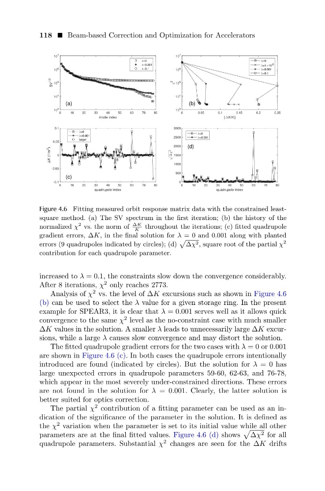
Figure 4.6 Fitting measured orbit response matrix data with the constrained leastsquare method. (a) The SV spectrum in the first iteration; (b) the history of the
normalized χ
2 vs. the norm of
∆K
K
throughout the iterations; (c) fitted quadrupole
gradient errors, ∆K, in the final solution for λ = 0 and 0.001 along with planted
errors (9 quadrupoles indicated by circles); (d)
∆χ 2 , square root of the partial χ
2
contribution for each quadrupole parameter.
increased to λ = 0.1, the constraints slow down the convergence considerably.
After 8 iterations, χ
2 only reaches 2773.
Analysis of χ
2 vs. the level of ∆K excursions such as shown in Figure 4.6
(b) can be used to select the λ value for a given storage ring. In the present
example for SPEAR3, it is clear that λ = 0.001 serves well as it allows quick
convergence to the same χ
2 level as the no-constraint case with much smaller
∆K values in the solution. A smaller λ leads to unnecessarily large ∆K excursions, while a large λ causes slow convergence and may distort the solution.
The fitted quadrupole gradient errors for the two cases with λ = 0 or 0.001
are shown in Figure 4.6 (c). In both cases the quadrupole errors intentionally
introduced are found (indicated by circles). But the solution for λ = 0 has
large unexpected errors in quadrupole parameters 59-60, 62-63, and 76-78,
which appear in the most severely under-constrained directions. These errors
are not found in the solution for λ = 0.001. Clearly, the latter solution is
better suited for optics correction.
The partial χ
2 contribution of a fitting parameter can be used as an indication of the significance of the parameter in the solution. It is defined as
the χ
2 variation when the parameter is set to its initial value while all other
parameters are at the final fitted values. Figure 4.6 (d) shows
∆χ 2 for all
quadrupole parameters. Substantial χ
2 changes are seen for the ∆K drifts
0
10
20
30
40
50
60
70
80
mode index
10 3
10 4
10 5
10 6
10 7
SV 1/2
(a)
=0
=0.001
=0.1
0
0.05
0.1
0.15
0.2
0.25
|| K/K||
10 3
10 4
10 5
10 6
10 7
2
(b)
=0
=1 10 -5
=0.001
=0.1
0
10
20
30
40
50
60
70
80
quadrupole index
-0.1
-0.05
0
0.05
0.1
K (1/m 2
)
(c)
=0
=0.001
target
0
10
20
30
40
50
60
70
80
quadrupole index
0
500
1000
1500
2000
2500
3000
(d)
=0
=0.001
Figure 4.6 Fitting measured orbit response matrix data with the constrained leastsquare method. (a) The SV spectrum in the first iteration; (b) the history of the
normalized χ
2 vs. the norm of
∆K
K
throughout the iterations; (c) fitted quadrupole
gradient errors, ∆K, in the final solution for λ = 0 and 0.001 along with planted
errors (9 quadrupoles indicated by circles); (d)
∆χ 2 , square root of the partial χ
2
contribution for each quadrupole parameter.
increased to λ = 0.1, the constraints slow down the convergence considerably.
After 8 iterations, χ
2 only reaches 2773.
Analysis of χ
2 vs. the level of ∆K excursions such as shown in Figure 4.6
(b) can be used to select the λ value for a given storage ring. In the present
example for SPEAR3, it is clear that λ = 0.001 serves well as it allows quick
convergence to the same χ
2 level as the no-constraint case with much smaller
∆K values in the solution. A smaller λ leads to unnecessarily large ∆K excursions, while a large λ causes slow convergence and may distort the solution.
The fitted quadrupole gradient errors for the two cases with λ = 0 or 0.001
are shown in Figure 4.6 (c). In both cases the quadrupole errors intentionally
introduced are found (indicated by circles). But the solution for λ = 0 has
large unexpected errors in quadrupole parameters 59-60, 62-63, and 76-78,
which appear in the most severely under-constrained directions. These errors
are not found in the solution for λ = 0.001. Clearly, the latter solution is
better suited for optics correction.
The partial χ
2 contribution of a fitting parameter can be used as an indication of the significance of the parameter in the solution. It is defined as
the χ
2 variation when the parameter is set to its initial value while all other
parameters are at the final fitted values. Figure 4.6 (d) shows
∆χ 2 for all
quadrupole parameters. Substantial χ
2 changes are seen for the ∆K drifts