

108 Beam-based Correction and Optimization for Accelerators
0
50
100
150
200
250
300
350
Index
10 0
10 2
10 4
10 6
SV
SV 306 <10 -11
1
2
3
4
5
6
7
8
Iteration
10 0
10 2
10 4
2
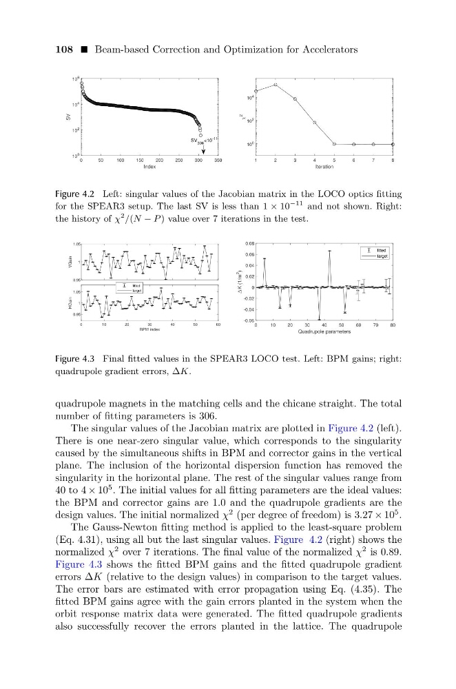
Figure 4.2 Left: singular values of the Jacobian matrix in the LOCO optics fitting
for the SPEAR3 setup. The last SV is less than 1 × 10
−11 and not shown. Right:
the history of χ
2 /(N − P ) value over 7 iterations in the test.
0.95
1
1.05
VGain
0
10
20
30
40
50
60
BPM index
0.95
1
1.05
HGain
fitted
target
0
10
20
30
40
50
60
70
80
Quadrupole parameters
-0.06
-0.04
-0.02
0
0.02
0.04
0.06
0.08
K (1/m
2
)
fitted
target
Figure 4.3 Final fitted values in the SPEAR3 LOCO test. Left: BPM gains; right:
quadrupole gradient errors, ∆K.
quadrupole magnets in the matching cells and the chicane straight. The total
number of fitting parameters is 306.
The singular values of the Jacobian matrix are plotted in Figure 4.2 (left).
There is one near-zero singular value, which corresponds to the singularity
caused by the simultaneous shifts in BPM and corrector gains in the vertical
plane. The inclusion of the horizontal dispersion function has removed the
singularity in the horizontal plane. The rest of the singular values range from
40 to 4 × 10
5 . The initial values for all fitting parameters are the ideal values:
the BPM and corrector gains are 1.0 and the quadrupole gradients are the
design values. The initial normalized χ
2 (per degree of freedom) is 3.27 × 10
5 .
The Gauss-Newton fitting method is applied to the least-square problem
(Eq. 4.31), using all but the last singular values. Figure 4.2 (right) shows the
normalized χ
2 over 7 iterations. The final value of the normalized χ
2 is 0.89.
Figure 4.3 shows the fitted BPM gains and the fitted quadrupole gradient
errors ∆K (relative to the design values) in comparison to the target values.
The error bars are estimated with error propagation using Eq. (4.35). The
fitted BPM gains agree with the gain errors planted in the system when the
orbit response matrix data were generated. The fitted quadrupole gradients
also successfully recover the errors planted in the lattice. The quadrupole
0
50
100
150
200
250
300
350
Index
10 0
10 2
10 4
10 6
SV
SV 306 <10 -11
1
2
3
4
5
6
7
8
Iteration
10 0
10 2
10 4
2
Figure 4.2 Left: singular values of the Jacobian matrix in the LOCO optics fitting
for the SPEAR3 setup. The last SV is less than 1 × 10
−11 and not shown. Right:
the history of χ
2 /(N − P ) value over 7 iterations in the test.
0.95
1
1.05
VGain
0
10
20
30
40
50
60
BPM index
0.95
1
1.05
HGain
fitted
target
0
10
20
30
40
50
60
70
80
Quadrupole parameters
-0.06
-0.04
-0.02
0
0.02
0.04
0.06
0.08
K (1/m
2
)
fitted
target
Figure 4.3 Final fitted values in the SPEAR3 LOCO test. Left: BPM gains; right:
quadrupole gradient errors, ∆K.
quadrupole magnets in the matching cells and the chicane straight. The total
number of fitting parameters is 306.
The singular values of the Jacobian matrix are plotted in Figure 4.2 (left).
There is one near-zero singular value, which corresponds to the singularity
caused by the simultaneous shifts in BPM and corrector gains in the vertical
plane. The inclusion of the horizontal dispersion function has removed the
singularity in the horizontal plane. The rest of the singular values range from
40 to 4 × 10
5 . The initial values for all fitting parameters are the ideal values:
the BPM and corrector gains are 1.0 and the quadrupole gradients are the
design values. The initial normalized χ
2 (per degree of freedom) is 3.27 × 10
5 .
The Gauss-Newton fitting method is applied to the least-square problem
(Eq. 4.31), using all but the last singular values. Figure 4.2 (right) shows the
normalized χ
2 over 7 iterations. The final value of the normalized χ
2 is 0.89.
Figure 4.3 shows the fitted BPM gains and the fitted quadrupole gradient
errors ∆K (relative to the design values) in comparison to the target values.
The error bars are estimated with error propagation using Eq. (4.35). The
fitted BPM gains agree with the gain errors planted in the system when the
orbit response matrix data were generated. The fitted quadrupole gradients
also successfully recover the errors planted in the lattice. The quadrupole