

Top Curr Chem (Z) (2018) 376:24
1 3
The ability to accurately predict ESA signals would then open the door for simulating broadband 2D electronic spectroscopy [37, 52–61] as well as double quantum
coherences spectroscopy [53, 62, 63].
As will be illustrated throughout Sect. 3, obtaining the electronic structure of biologically relevant chromophores from first principles, at a level of accuracy needed
for comparison against experimental data, is far from trivial. A protocol for computing reliable TEs and TDMs of isolated bio-chromophores (or dimeric aggregates) is
presented in Sect. 3.1, which comes with additional benefits: (a) the results can be
used to expand currently available exciton models beyond the lowest transitions; (b)
the results can be used to benchmark low-cost approaches that can then be applied
for larger-scale computations; (c) the results essentially make simulations independent from the experiment, providing them with predictive power and allowing us to
envision problem-driven experimental setups. To this aim, we take a step back in the
theoretical descriptions given in Sect. 2.2 and start from a drastic approximation, i.e.
treating the chromophoric system uncoupled from the bath of vibrations and thus
as a closed quantum system having only electronic degrees of freedom. Within this
framework the electronic states become eigenstates of the system’s Hamiltonian,
and their dynamics are reduced to a e
−i f t
phase factor (herein referred to as a “static
picture”).
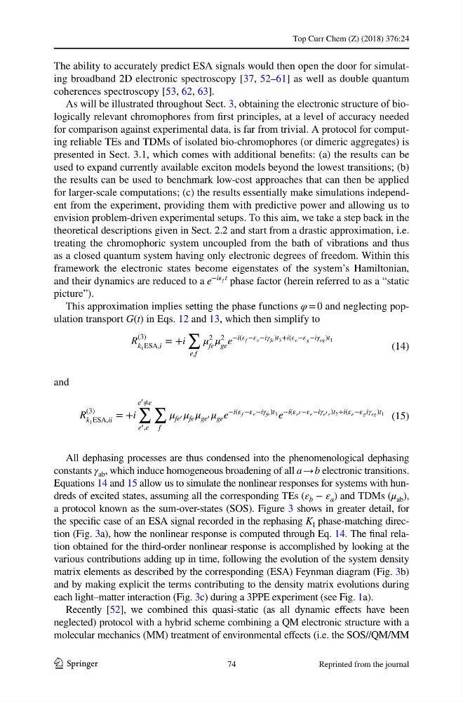
This approximation implies setting the phase functions φ = 0 and neglecting population transport G(t) in Eqs. 12 and 13, which then simplify to
and
All dephasing processes are thus condensed into the phenomenological dephasing
constants γ ab , which induce homogeneous broadening of all a → b electronic transitions.
Equations 14 and 15 allow us to simulate the nonlinear responses for systems with hundreds of excited states, assuming all the corresponding TEs (ε b − ε a ) and TDMs (μ ab ),
a protocol known as the sum-over-states (SOS). Figure 3 shows in greater detail, for
the specific case of an ESA signal recorded in the rephasing K I phase-matching direction (Fig. 3a), how the nonlinear response is computed through Eq. 14. The final relation obtained for the third-order nonlinear response is accomplished by looking at the
various contributions adding up in time, following the evolution of the system density
matrix elements as described by the corresponding (ESA) Feynman diagram (Fig. 3b)
and by making explicit the terms contributing to the density matrix evolutions during
each light–matter interaction (Fig. 3c) during a 3PPE experiment (see Fig. 1a).
Recently [52], we combined this quasi-static (as all dynamic effects have been
neglected) protocol with a hybrid scheme combining a QM electronic structure with a
molecular mechanics (MM) treatment of environmental effects (i.e. the SOS//QM/MM
(14)
R
(3)
k 1 ESA,i
= +i
∑
e,f
2
fe
2
ge
e
−i( f − e −i fe )t 3 +i( e − g −i eg )t 1
(15)
R
(3)
k 1 ESA,ii
= +i
e � ≠e
∑
e � ,e
∑
f
fe � fe ge � ge e
−i( f − e −i fe )t 3 e
−i( e � − e −i e � e )t 2 +i( e − g i eg )t 1
74
Reprinted from the journal
1 3
The ability to accurately predict ESA signals would then open the door for simulating broadband 2D electronic spectroscopy [37, 52–61] as well as double quantum
coherences spectroscopy [53, 62, 63].
As will be illustrated throughout Sect. 3, obtaining the electronic structure of biologically relevant chromophores from first principles, at a level of accuracy needed
for comparison against experimental data, is far from trivial. A protocol for computing reliable TEs and TDMs of isolated bio-chromophores (or dimeric aggregates) is
presented in Sect. 3.1, which comes with additional benefits: (a) the results can be
used to expand currently available exciton models beyond the lowest transitions; (b)
the results can be used to benchmark low-cost approaches that can then be applied
for larger-scale computations; (c) the results essentially make simulations independent from the experiment, providing them with predictive power and allowing us to
envision problem-driven experimental setups. To this aim, we take a step back in the
theoretical descriptions given in Sect. 2.2 and start from a drastic approximation, i.e.
treating the chromophoric system uncoupled from the bath of vibrations and thus
as a closed quantum system having only electronic degrees of freedom. Within this
framework the electronic states become eigenstates of the system’s Hamiltonian,
and their dynamics are reduced to a e
−i f t
phase factor (herein referred to as a “static
picture”).
This approximation implies setting the phase functions φ = 0 and neglecting population transport G(t) in Eqs. 12 and 13, which then simplify to
and
All dephasing processes are thus condensed into the phenomenological dephasing
constants γ ab , which induce homogeneous broadening of all a → b electronic transitions.
Equations 14 and 15 allow us to simulate the nonlinear responses for systems with hundreds of excited states, assuming all the corresponding TEs (ε b − ε a ) and TDMs (μ ab ),
a protocol known as the sum-over-states (SOS). Figure 3 shows in greater detail, for
the specific case of an ESA signal recorded in the rephasing K I phase-matching direction (Fig. 3a), how the nonlinear response is computed through Eq. 14. The final relation obtained for the third-order nonlinear response is accomplished by looking at the
various contributions adding up in time, following the evolution of the system density
matrix elements as described by the corresponding (ESA) Feynman diagram (Fig. 3b)
and by making explicit the terms contributing to the density matrix evolutions during
each light–matter interaction (Fig. 3c) during a 3PPE experiment (see Fig. 1a).
Recently [52], we combined this quasi-static (as all dynamic effects have been
neglected) protocol with a hybrid scheme combining a QM electronic structure with a
molecular mechanics (MM) treatment of environmental effects (i.e. the SOS//QM/MM
(14)
R
(3)
k 1 ESA,i
= +i
∑
e,f
2
fe
2
ge
e
−i( f − e −i fe )t 3 +i( e − g −i eg )t 1
(15)
R
(3)
k 1 ESA,ii
= +i
e � ≠e
∑
e � ,e
∑
f
fe � fe ge � ge e
−i( f − e −i fe )t 3 e
−i( e � − e −i e � e )t 2 +i( e − g i eg )t 1
74
Reprinted from the journal