

upon successive excitation and the color-coding will become clear in what follows.
In the pulse sequence shown in Fig. 2, the first pulse (E 1 ) acts on the sample and
induces a vibrational coherence between the |0i and |1i levels (oscillatory line).
Followed by a certain time t 1 , the so-called coherence time, a second laser pulse (E 2 )
converts this coherence into a population state, e.g. in |1i, which afterwards decays
during vibrational relaxation taking place during the waiting time t 2 , the so-called
population time. The evolution of the system is interrogated by the help of a third
field (E 3 ), which again induces a vibrational coherence that oscillates during the
time t 3 and that may be generated between levels |0i and |1i, or |1i and |2i. The local
oscillator (E LO ) does not interact with the sample and is only used for heterodyne
detection.
To generate two frequency axes for the 2D IR data, two Fourier transformations
are necessary for obtaining the ‘‘pump’’ and the ‘‘probe’’ axis. The first Fourier
transformation is generally performed by a detector, on which the signal light is
spectrally resolved. This generates the probe spectral axis, just as in ordinary
transient absorption spectroscopy. To obtain the pump spectral axis, the delay t 1
between the first two pulses is successively scanned, thereby mapping out the
evolution of the coherence generated by the first field interaction. If the fields E 1 and
E 2 have a fixed phase relation, such a scan results in an oscillatory signal along the
t 1 axis, which, after Fourier transformation yields the pump spectral axis
[10, 49, 61].
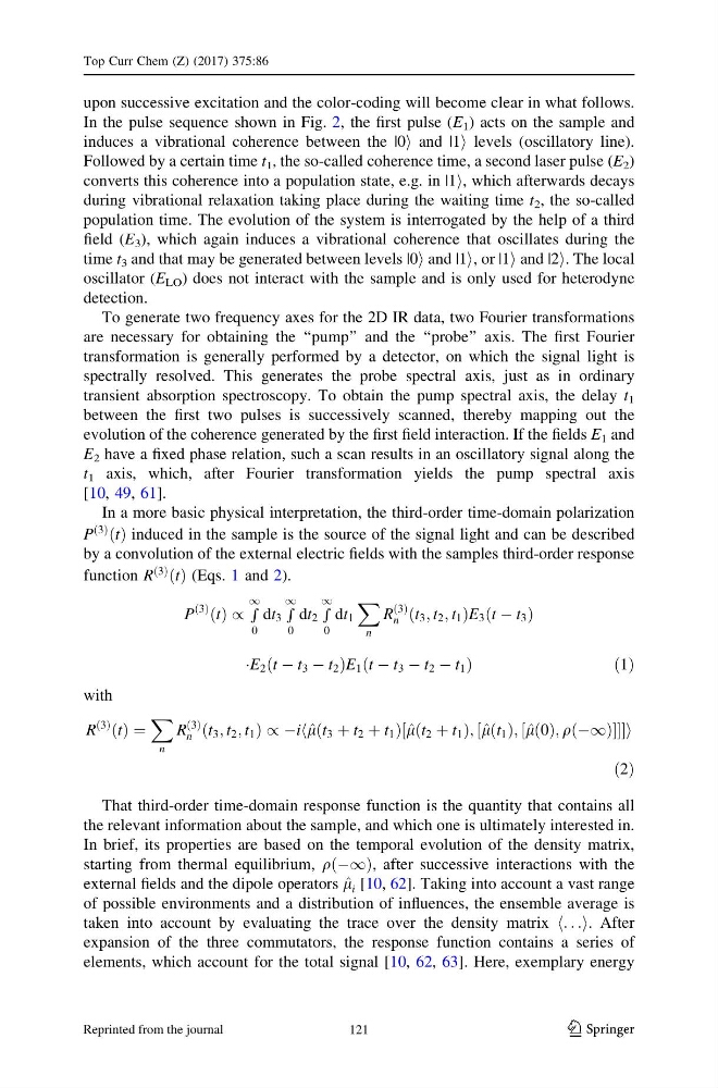
In a more basic physical interpretation, the third-order time-domain polarization
P
3
ð Þ t
ð Þ induced in the sample is the source of the signal light and can be described
by a convolution of the external electric fields with the samples third-order response
function R
3
ð Þ t
ð Þ (Eqs. 1 and 2).
P
3
ð Þ t
ð Þ / r
1
0
dt 3 r
1
0
dt 2 r
1
0
dt 1
X
n
R
3
ð Þ
n t 3 ; t 2 ; t 1
ð
ÞE 3 t À t 3
ð
Þ
ÁE 2 t À t 3 À t 2
ð
Þ E 1 t À t 3 À t 2 À t 1
ð
Þ
ð 1Þ
with
R
3
ð Þ t
ð Þ ¼
X
n
R
3
ð Þ
n t 3 ; t 2 ; t 1
ð
Þ/Àih ^
l t 3 þ t 2 þ t 1
ð
Þ^ l t 2 þ t 1
ð
Þ; ^
l t 1
ð Þ; ^
l 0
ð Þ; q À1
ð
Þ
½
½
½
i
ð2Þ
That third-order time-domain response function is the quantity that contains all
the relevant information about the sample, and which one is ultimately interested in.
In brief, its properties are based on the temporal evolution of the density matrix,
starting from thermal equilibrium, q À1
ð
Þ, after successive interactions with the
external fields and the dipole operators ^
l i [10, 62]. Taking into account a vast range
of possible environments and a distribution of influences, the ensemble average is
taken into account by evaluating the trace over the density matrix h. . .i. After
expansion of the three commutators, the response function contains a series of
elements, which account for the total signal [10, 62, 63]. Here, exemplary energy
Top Curr Chem (Z) (2017) 375:86
123
121
Reprinted from the journal
In the pulse sequence shown in Fig. 2, the first pulse (E 1 ) acts on the sample and
induces a vibrational coherence between the |0i and |1i levels (oscillatory line).
Followed by a certain time t 1 , the so-called coherence time, a second laser pulse (E 2 )
converts this coherence into a population state, e.g. in |1i, which afterwards decays
during vibrational relaxation taking place during the waiting time t 2 , the so-called
population time. The evolution of the system is interrogated by the help of a third
field (E 3 ), which again induces a vibrational coherence that oscillates during the
time t 3 and that may be generated between levels |0i and |1i, or |1i and |2i. The local
oscillator (E LO ) does not interact with the sample and is only used for heterodyne
detection.
To generate two frequency axes for the 2D IR data, two Fourier transformations
are necessary for obtaining the ‘‘pump’’ and the ‘‘probe’’ axis. The first Fourier
transformation is generally performed by a detector, on which the signal light is
spectrally resolved. This generates the probe spectral axis, just as in ordinary
transient absorption spectroscopy. To obtain the pump spectral axis, the delay t 1
between the first two pulses is successively scanned, thereby mapping out the
evolution of the coherence generated by the first field interaction. If the fields E 1 and
E 2 have a fixed phase relation, such a scan results in an oscillatory signal along the
t 1 axis, which, after Fourier transformation yields the pump spectral axis
[10, 49, 61].
In a more basic physical interpretation, the third-order time-domain polarization
P
3
ð Þ t
ð Þ induced in the sample is the source of the signal light and can be described
by a convolution of the external electric fields with the samples third-order response
function R
3
ð Þ t
ð Þ (Eqs. 1 and 2).
P
3
ð Þ t
ð Þ / r
1
0
dt 3 r
1
0
dt 2 r
1
0
dt 1
X
n
R
3
ð Þ
n t 3 ; t 2 ; t 1
ð
ÞE 3 t À t 3
ð
Þ
ÁE 2 t À t 3 À t 2
ð
Þ E 1 t À t 3 À t 2 À t 1
ð
Þ
ð 1Þ
with
R
3
ð Þ t
ð Þ ¼
X
n
R
3
ð Þ
n t 3 ; t 2 ; t 1
ð
Þ/Àih ^
l t 3 þ t 2 þ t 1
ð
Þ^ l t 2 þ t 1
ð
Þ; ^
l t 1
ð Þ; ^
l 0
ð Þ; q À1
ð
Þ
½
½
½
i
ð2Þ
That third-order time-domain response function is the quantity that contains all
the relevant information about the sample, and which one is ultimately interested in.
In brief, its properties are based on the temporal evolution of the density matrix,
starting from thermal equilibrium, q À1
ð
Þ, after successive interactions with the
external fields and the dipole operators ^
l i [10, 62]. Taking into account a vast range
of possible environments and a distribution of influences, the ensemble average is
taken into account by evaluating the trace over the density matrix h. . .i. After
expansion of the three commutators, the response function contains a series of
elements, which account for the total signal [10, 62, 63]. Here, exemplary energy
Top Curr Chem (Z) (2017) 375:86
123
121
Reprinted from the journal