

Top Curr Chem (Z) (2018) 376:24
1 3
homogeneous line broadening, and (ii) decay and simultaneous buildup of spectral signatures, the former process being associated with the population decrease
in the initial state, the latter with the population growth in the final state. The
CGF framework offers a prescript for incorporating population transfer, i.e. the socalled doorway–window (DW) factorization [100, 101]. When dephasing is much
faster compared to transport, the secular Redfield approximation can be applied,
providing separate expressions for coherences (Eq. 13) and populations (Eq. 12).
Correlated bath dynamics in the coherence is described with the phase function
e � fe ( 4 , 3 , 2 , 1 ) introduced in the previous section (Eq. 16). In contrast, when
bath fluctuations decay more slowly than the coherence dephasing but faster than
population transport, the population term (in Eq. 13) can be treated by applying
the Markovian approximation to the time intervals between the pulses, with the
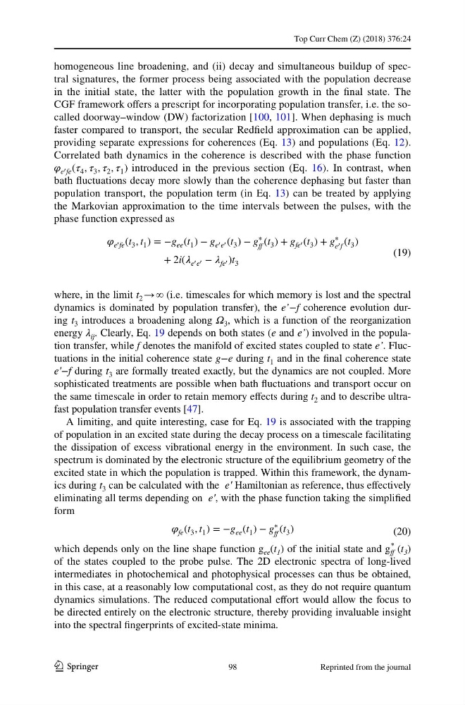
phase function expressed as
where, in the limit t 2 → ∞ (i.e. timescales for which memory is lost and the spectral
dynamics is dominated by population transfer), the e’−f coherence evolution during t 3 introduces a broadening along Ω 3 , which is a function of the reorganization
energy λ ij . Clearly, Eq. 19 depends on both states (e and e’) involved in the population transfer, while f denotes the manifold of excited states coupled to state e’. Fluctuations in the initial coherence state g−e during t 1 and in the final coherence state
e′−f during t 3 are formally treated exactly, but the dynamics are not coupled. More
sophisticated treatments are possible when bath fluctuations and transport occur on
the same timescale in order to retain memory effects during t 2 and to describe ultrafast population transfer events [47].
A limiting, and quite interesting, case for Eq. 19 is associated with the trapping
of population in an excited state during the decay process on a timescale facilitating
the dissipation of excess vibrational energy in the environment. In such case, the
spectrum is dominated by the electronic structure of the equilibrium geometry of the
excited state in which the population is trapped. Within this framework, the dynamics during t 3 can be calculated with the e′ Hamiltonian as reference, thus effectively
eliminating all terms depending on e′, with the phase function taking the simplified
form
which depends only on the line shape function g ee (t 1 ) of the initial state and g ff
*
(t 3 )
of the states coupled to the probe pulse. The 2D electronic spectra of long-lived
intermediates in photochemical and photophysical processes can thus be obtained,
in this case, at a reasonably low computational cost, as they do not require quantum
dynamics simulations. The reduced computational effort would allow the focus to
be directed entirely on the electronic structure, thereby providing invaluable insight
into the spectral fingerprints of excited-state minima.
(19)
e � fe (t 3 , t 1 ) = −g ee (t 1 ) − g e � e � (t 3 ) − g
∗
ff (t 3 ) + g fe � (t 3 ) + g
∗
e � f (t 3 )
+ 2i( e � e � − fe � )t 3
(20)
fe (t 3 , t 1 ) = −g ee (t 1 ) − g
∗
ff
(t 3 )
98
Reprinted from the journal
1 3
homogeneous line broadening, and (ii) decay and simultaneous buildup of spectral signatures, the former process being associated with the population decrease
in the initial state, the latter with the population growth in the final state. The
CGF framework offers a prescript for incorporating population transfer, i.e. the socalled doorway–window (DW) factorization [100, 101]. When dephasing is much
faster compared to transport, the secular Redfield approximation can be applied,
providing separate expressions for coherences (Eq. 13) and populations (Eq. 12).
Correlated bath dynamics in the coherence is described with the phase function
e � fe ( 4 , 3 , 2 , 1 ) introduced in the previous section (Eq. 16). In contrast, when
bath fluctuations decay more slowly than the coherence dephasing but faster than
population transport, the population term (in Eq. 13) can be treated by applying
the Markovian approximation to the time intervals between the pulses, with the
phase function expressed as
where, in the limit t 2 → ∞ (i.e. timescales for which memory is lost and the spectral
dynamics is dominated by population transfer), the e’−f coherence evolution during t 3 introduces a broadening along Ω 3 , which is a function of the reorganization
energy λ ij . Clearly, Eq. 19 depends on both states (e and e’) involved in the population transfer, while f denotes the manifold of excited states coupled to state e’. Fluctuations in the initial coherence state g−e during t 1 and in the final coherence state
e′−f during t 3 are formally treated exactly, but the dynamics are not coupled. More
sophisticated treatments are possible when bath fluctuations and transport occur on
the same timescale in order to retain memory effects during t 2 and to describe ultrafast population transfer events [47].
A limiting, and quite interesting, case for Eq. 19 is associated with the trapping
of population in an excited state during the decay process on a timescale facilitating
the dissipation of excess vibrational energy in the environment. In such case, the
spectrum is dominated by the electronic structure of the equilibrium geometry of the
excited state in which the population is trapped. Within this framework, the dynamics during t 3 can be calculated with the e′ Hamiltonian as reference, thus effectively
eliminating all terms depending on e′, with the phase function taking the simplified
form
which depends only on the line shape function g ee (t 1 ) of the initial state and g ff
*
(t 3 )
of the states coupled to the probe pulse. The 2D electronic spectra of long-lived
intermediates in photochemical and photophysical processes can thus be obtained,
in this case, at a reasonably low computational cost, as they do not require quantum
dynamics simulations. The reduced computational effort would allow the focus to
be directed entirely on the electronic structure, thereby providing invaluable insight
into the spectral fingerprints of excited-state minima.
(19)
e � fe (t 3 , t 1 ) = −g ee (t 1 ) − g e � e � (t 3 ) − g
∗
ff (t 3 ) + g fe � (t 3 ) + g
∗
e � f (t 3 )
+ 2i( e � e � − fe � )t 3
(20)
fe (t 3 , t 1 ) = −g ee (t 1 ) − g
∗
ff
(t 3 )
98
Reprinted from the journal