

499
σ
ε
ij
σ
ij
ε
W
=
∂
∂
(1)
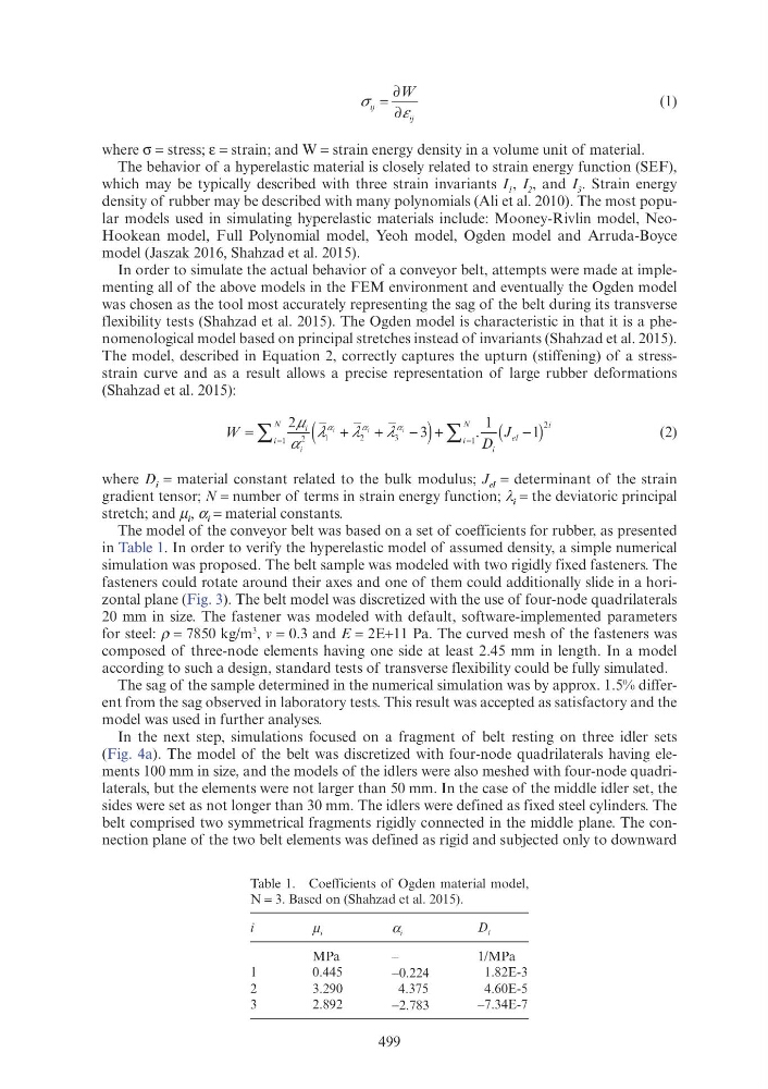
where σ = stress; ε = strain; and W = strain energy density in a volume unit of material.
The behavior of a hyperelastic material is closely related to strain energy function (SEF),
which may be typically described with three strain invariants I 1 , I 2 , and I 3 . Strain energy
density of rubber may be described with many polynomials (Ali et al. 2010). The most popular models used in simulating hyperelastic materials include: Mooney-Rivlin model, NeoHookean model, Full Polynomial model, Yeoh model, Ogden model and Arruda-Boyce
model (Jaszak 2016, Shahzad et al. 2015).
In order to simulate the actual behavior of a conveyor belt, attempts were made at implementing all of the above models in the FEM environment and eventually the Ogden model
was chosen as the tool most accurately representing the sag of the belt during its transverse
flexibility tests (Shahzad et al. 2015). The Ogden model is characteristic in that it is a phenomenological model based on principal stretches instead of invariants (Shahzad et al. 2015).
The model, described in Equation 2, correctly captures the upturn (stiffening) of a stressstrain curve and as a result allows a precise representation of large rubber deformations
(Shahzad et al. 2015):
D
i
i
N
i
N
i
D
i
=
(
)
(
)
J el
J −
J el
J
=
i
∑
∑
i
i
N
∑
(
)
i
−
i
+
=
(
)
2
1
1
1
2
μ i i
α i
i
+
+
+
i i i
+
i i
i
i
i i i i
.
(2)
where D i = material constant related to the bulk modulus; J el = determinant of the strain
gradient tensor; N = number of terms in strain energy function; λ i = the deviatoric principal
stretch; and μ i , α i = material constants.
The model of the conveyor belt was based on a set of coefficients for rubber, as presented
in Table 1. In order to verify the hyperelastic model of assumed density, a simple numerical
simulation was proposed. The belt sample was modeled with two rigidly fixed fasteners. The
fasteners could rotate around their axes and one of them could additionally slide in a horizontal plane (Fig. 3). The belt model was discretized with the use of four-node quadrilaterals
20 mm in size. The fastener was modeled with default, software-implemented parameters
for steel: ρ = 7850 kg/m
3
, v = 0.3 and E = 2E+11 Pa. The curved mesh of the fasteners was
composed of three-node elements having one side at least 2.45 mm in length. In a model
according to such a design, standard tests of transverse flexibility could be fully simulated.
The sag of the sample determined in the numerical simulation was by approx. 1.5% different from the sag observed in laboratory tests. This result was accepted as satisfactory and the
model was used in further analyses.
In the next step, simulations focused on a fragment of belt resting on three idler sets
(Fig. 4a). The model of the belt was discretized with four-node quadrilaterals having elements 100 mm in size, and the models of the idlers were also meshed with four-node quadrilaterals, but the elements were not larger than 50 mm. In the case of the middle idler set, the
sides were set as not longer than 30 mm. The idlers were defined as fixed steel cylinders. The
belt comprised two symmetrical fragments rigidly connected in the middle plane. The connection plane of the two belt elements was defined as rigid and subjected only to downward
Table 1. Coefficients of Ogden material model,
N = 3. Based on (Shahzad et al. 2015).
i
μ i
α i
D i
MPa
–
1/MPa
1
0.445
−0.224
1.82E-3
2
3.290
4.375
4.60E-5
3
2.892
−2.783
–7.34E-7
σ
ε
ij
σ
ij
ε
W
=
∂
∂
(1)
where σ = stress; ε = strain; and W = strain energy density in a volume unit of material.
The behavior of a hyperelastic material is closely related to strain energy function (SEF),
which may be typically described with three strain invariants I 1 , I 2 , and I 3 . Strain energy
density of rubber may be described with many polynomials (Ali et al. 2010). The most popular models used in simulating hyperelastic materials include: Mooney-Rivlin model, NeoHookean model, Full Polynomial model, Yeoh model, Ogden model and Arruda-Boyce
model (Jaszak 2016, Shahzad et al. 2015).
In order to simulate the actual behavior of a conveyor belt, attempts were made at implementing all of the above models in the FEM environment and eventually the Ogden model
was chosen as the tool most accurately representing the sag of the belt during its transverse
flexibility tests (Shahzad et al. 2015). The Ogden model is characteristic in that it is a phenomenological model based on principal stretches instead of invariants (Shahzad et al. 2015).
The model, described in Equation 2, correctly captures the upturn (stiffening) of a stressstrain curve and as a result allows a precise representation of large rubber deformations
(Shahzad et al. 2015):
D
i
i
N
i
N
i
D
i
=
(
)
(
)
J el
J −
J el
J
=
i
∑
∑
i
i
N
∑
(
)
i
−
i
+
=
(
)
2
1
1
1
2
μ i i
α i
i
+
+
+
i i i
+
i i
i
i
i i i i
.
(2)
where D i = material constant related to the bulk modulus; J el = determinant of the strain
gradient tensor; N = number of terms in strain energy function; λ i = the deviatoric principal
stretch; and μ i , α i = material constants.
The model of the conveyor belt was based on a set of coefficients for rubber, as presented
in Table 1. In order to verify the hyperelastic model of assumed density, a simple numerical
simulation was proposed. The belt sample was modeled with two rigidly fixed fasteners. The
fasteners could rotate around their axes and one of them could additionally slide in a horizontal plane (Fig. 3). The belt model was discretized with the use of four-node quadrilaterals
20 mm in size. The fastener was modeled with default, software-implemented parameters
for steel: ρ = 7850 kg/m
3
, v = 0.3 and E = 2E+11 Pa. The curved mesh of the fasteners was
composed of three-node elements having one side at least 2.45 mm in length. In a model
according to such a design, standard tests of transverse flexibility could be fully simulated.
The sag of the sample determined in the numerical simulation was by approx. 1.5% different from the sag observed in laboratory tests. This result was accepted as satisfactory and the
model was used in further analyses.
In the next step, simulations focused on a fragment of belt resting on three idler sets
(Fig. 4a). The model of the belt was discretized with four-node quadrilaterals having elements 100 mm in size, and the models of the idlers were also meshed with four-node quadrilaterals, but the elements were not larger than 50 mm. In the case of the middle idler set, the
sides were set as not longer than 30 mm. The idlers were defined as fixed steel cylinders. The
belt comprised two symmetrical fragments rigidly connected in the middle plane. The connection plane of the two belt elements was defined as rigid and subjected only to downward
Table 1. Coefficients of Ogden material model,
N = 3. Based on (Shahzad et al. 2015).
i
μ i
α i
D i
MPa
–
1/MPa
1
0.445
−0.224
1.82E-3
2
3.290
4.375
4.60E-5
3
2.892
−2.783
–7.34E-7