

464
as described by Carrasco et al. (2008), “quantities are said to be additive if the averaged
quantity equals the average of the quantities”. The non-additivity of an attribute refrains
the use linear averages as it would generate biased or inconsistent results according to the
studied phenomenon.
One of the most applied techniques to forecast geometallurgical variables is linear regression analysis, uni or multivariate, which uses as independent variables information about in
situ ore, including grade, grain size distribution or lithology to predict variables such as ore
recovery at the processing plant. Examples using this technique in geometallurgy modelling
are found in MacMillan et al. (2011), Montoya et al. (2011), Fernandes (2013), Motta (2014),
Vieira (2016), among others. Despite of frequently show good results when applied to forecast geometallurgical variables, when regression models are used to estimate variables which
complement themselves, as mass and metallurgical recoveries modeled at each plant output,
it is known that not necessarily the predictions sum will bring a perfect closure. Furthermore,
once it is a linear estimation, its use to forecast non-additive variables can generate results
that do not represent ideally the phenomenon studied.
One alternative to the application of regression analysis, able to overcome the problems
describe above, is by using neural networks. Once it uses non-linear activation functions,
its use to model non-additive variables is ideal. Another advantage of neural networks is its
capacity to estimate simultaneously two or more dependent variables, reducing time during
the geometallurgical model elaboration. To compare the results achieved using both techniques herein cited, Nexa Resources provided a database with 49 geometallurgical samples
collected at Vazante mine, located in Minas Gerais state, Brazil. The plant under study
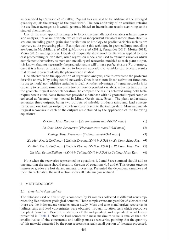
generates three outputs, being two outputs of saleable products (zinc and lead concentrates) and one tailings output, which are directly sent to the tailings dam. Mass and metallurgical recoveries in each of the outputs are obtained by the application of the following
equations:
Conc
y
. Mass Recovery r (
)
ROM mass
/
Zn c
Z Z oncentrate mass R
s
(1)
Pb Conc
y
. Mass Recovery r (
)
ROM mass
/
Pb concentrate mass R
s
(2)
Tailings Mass Recovery r (
)
Tailings T T
mass ROM mass
s s R
(3)
Zn Met Rec in Zn Conc
Mass Rec
.
.
Rec
.
.
x Zn Conc
(
)
in Zn conc Zn
%
Zn
. /Z % in ROM
. . (4)
Zn Met Rec in Pb Conc
b
Mass Rec
.
.
Rec
.
.
x Pb Conc
(
)
in Pb conc Zn
%
Zn
. /Z % in ROM
. . (5)
Zn Met Rec in Tailings
x Tailings Mass
.
.
Rec
= (
)
Zn
g Zn in ROM
%
/
in Tailings s Z %
Re R R c.
(6)
Note when the recoveries represented on equations 1, 2 and 3 are summed should add to
one and that the same should result to the sum of equations 4, 5 and 6. This occurs once no
masses or grades are lost during mineral processing. Presented the dependent variables and
their characteristics, the next section shows all data analysis realized.
2 METHODOLOGY
2.1 Descriptive data analysis
The database used on this study is composed by 49 samples collected at different zones representing five different geological domains. These samples were analyzed for 28 elements and
those are the independent variables under study. Mass and zinc metallurgical recoveries in
tailings, zinc and lead concentrates were obtained through flotation tests which reproduce
the plant flowchart. Descriptive statistics of the independent and dependent variables are
presented in Table 1. Note the lead concentrate mass maximum value is smaller than the
smallest value of zinc concentrate and tailings masses recoveries, pointing that the quantity
of this material generated by the plant represents a really small portion of the mass processed.
as described by Carrasco et al. (2008), “quantities are said to be additive if the averaged
quantity equals the average of the quantities”. The non-additivity of an attribute refrains
the use linear averages as it would generate biased or inconsistent results according to the
studied phenomenon.
One of the most applied techniques to forecast geometallurgical variables is linear regression analysis, uni or multivariate, which uses as independent variables information about in
situ ore, including grade, grain size distribution or lithology to predict variables such as ore
recovery at the processing plant. Examples using this technique in geometallurgy modelling
are found in MacMillan et al. (2011), Montoya et al. (2011), Fernandes (2013), Motta (2014),
Vieira (2016), among others. Despite of frequently show good results when applied to forecast geometallurgical variables, when regression models are used to estimate variables which
complement themselves, as mass and metallurgical recoveries modeled at each plant output,
it is known that not necessarily the predictions sum will bring a perfect closure. Furthermore,
once it is a linear estimation, its use to forecast non-additive variables can generate results
that do not represent ideally the phenomenon studied.
One alternative to the application of regression analysis, able to overcome the problems
describe above, is by using neural networks. Once it uses non-linear activation functions,
its use to model non-additive variables is ideal. Another advantage of neural networks is its
capacity to estimate simultaneously two or more dependent variables, reducing time during
the geometallurgical model elaboration. To compare the results achieved using both techniques herein cited, Nexa Resources provided a database with 49 geometallurgical samples
collected at Vazante mine, located in Minas Gerais state, Brazil. The plant under study
generates three outputs, being two outputs of saleable products (zinc and lead concentrates) and one tailings output, which are directly sent to the tailings dam. Mass and metallurgical recoveries in each of the outputs are obtained by the application of the following
equations:
Conc
y
. Mass Recovery r (
)
ROM mass
/
Zn c
Z Z oncentrate mass R
s
(1)
Pb Conc
y
. Mass Recovery r (
)
ROM mass
/
Pb concentrate mass R
s
(2)
Tailings Mass Recovery r (
)
Tailings T T
mass ROM mass
s s R
(3)
Zn Met Rec in Zn Conc
Mass Rec
.
.
Rec
.
.
x Zn Conc
(
)
in Zn conc Zn
%
Zn
. /Z % in ROM
. . (4)
Zn Met Rec in Pb Conc
b
Mass Rec
.
.
Rec
.
.
x Pb Conc
(
)
in Pb conc Zn
%
Zn
. /Z % in ROM
. . (5)
Zn Met Rec in Tailings
x Tailings Mass
.
.
Rec
= (
)
Zn
g Zn in ROM
%
/
in Tailings s Z %
Re R R c.
(6)
Note when the recoveries represented on equations 1, 2 and 3 are summed should add to
one and that the same should result to the sum of equations 4, 5 and 6. This occurs once no
masses or grades are lost during mineral processing. Presented the dependent variables and
their characteristics, the next section shows all data analysis realized.
2 METHODOLOGY
2.1 Descriptive data analysis
The database used on this study is composed by 49 samples collected at different zones representing five different geological domains. These samples were analyzed for 28 elements and
those are the independent variables under study. Mass and zinc metallurgical recoveries in
tailings, zinc and lead concentrates were obtained through flotation tests which reproduce
the plant flowchart. Descriptive statistics of the independent and dependent variables are
presented in Table 1. Note the lead concentrate mass maximum value is smaller than the
smallest value of zinc concentrate and tailings masses recoveries, pointing that the quantity
of this material generated by the plant represents a really small portion of the mass processed.