332
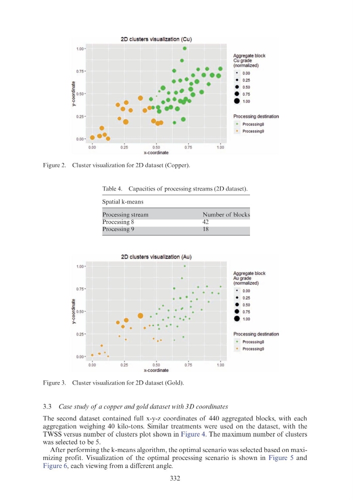
Table 4. Capacities of processing streams (2D dataset).
Spatial k-means
Processing stream
Number of blocks
Processing 8
42
Processing 9
18
Figure 2. Cluster visualization for 2D dataset (Copper).
Figure 3. Cluster visualization for 2D dataset (Gold).
3.3 Case study of a copper and gold dataset with 3D coordinates
The second dataset contained full x-y-z coordinates of 440 aggregated blocks, with each
aggregation weighing 40 kilo-tons. Similar treatments were used on the dataset, with the
TWSS versus number of clusters plot shown in Figure 4. The maximum number of clusters
was selected to be 5.
After performing the k-means algorithm, the optimal scenario was selected based on maximizing profit. Visualization of the optimal processing scenario is shown in Figure  5 and
Figure 6, each viewing from a different angle.
1.00 -
0.75 -
2 ., c
~ 0.50 -
0
u
>.
~ c
0.25 -
o.oo -
1.00 -
0.75 -
~ 0500
u
>.
0.25 -
0.00 -
•
••••
0.00
•
• •
0.00
20 clusters visualization (Cu)
•
•• ••
••
0.25
•
• • ••
••••
••••• •
.• ... ~.
...... .,.
.. . , ...
... ..
0.50
x-coordinate
0.75
1.00
20 clusters visualization (Au)
•• • •
0.25
•
•
. . .
. ,
. . .
. . .
•
. . . ...
...
0.50
x-coordinate
0.75
. .
1.00
Aggreg ate block
Cu grade
(normalized)
0.00
• 0.25
•
0.50
•
0.75
•
1.00
Processing destination
• ProcessingS
• Processing9
Aggregate block
Au grade
(normalized)
0.00
• 0.25
•
0.50
•
0.75
•
1.00
Processing destination
• Processing8
• Processing9