

306
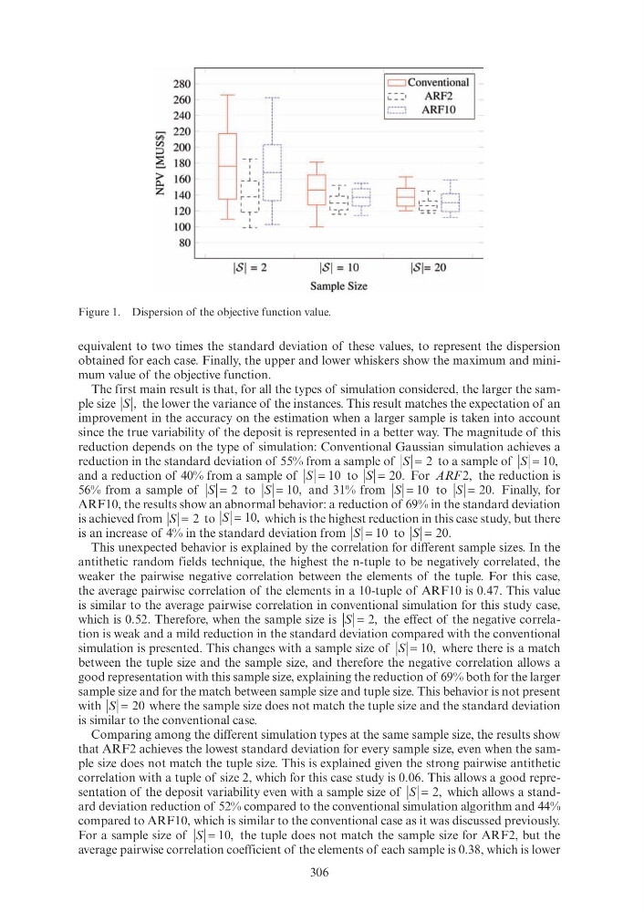
equivalent to two times the standard deviation of these values, to represent the dispersion
obtained for each case. Finally, the upper and lower whiskers show the maximum and minimum value of the objective function.
The first main result is that, for all the types of simulation considered, the larger the sample size S , the lower the variance of the instances. This result matches the expectation of an
improvement in the accuracy on the estimation when a larger sample is taken into account
since the true variability of the deposit is represented in a better way. The magnitude of this
reduction depends on the type of simulation: Conventional Gaussian simulation achieves a
reduction in the standard deviation of 55% from a sample of S = 2 to a sample of S = 10,
and a reduction of 40% from a sample of S = 10 to S = 20. For ARF 2, the reduction is
56% from a sample of S = 2 to S = 10, and 31% from S = 10 to S = 20. Finally, for
ARF10, the results show an abnormal behavior: a reduction of 69% in the standard deviation
is achieved from S = 2 to S = 10, which is the highest reduction in this case study, but there
is an increase of 4% in the standard deviation from S = 10 to S = 20.
This unexpected behavior is explained by the correlation for different sample sizes. In the
antithetic random fields technique, the highest the n-tuple to be negatively correlated, the
weaker the pairwise negative correlation between the elements of the tuple. For this case,
the average pairwise correlation of the elements in a 10-tuple of ARF10 is 0.47. This value
is similar to the average pairwise correlation in conventional simulation for this study case,
which is 0.52. Therefore, when the sample size is S = 2, the effect of the negative correlation is weak and a mild reduction in the standard deviation compared with the conventional
simulation is presented. This changes with a sample size of S = 10, where there is a match
between the tuple size and the sample size, and therefore the negative correlation allows a
good representation with this sample size, explaining the reduction of 69% both for the larger
sample size and for the match between sample size and tuple size. This behavior is not present
with S = 20 where the sample size does not match the tuple size and the standard deviation
is similar to the conventional case.
Comparing among the different simulation types at the same sample size, the results show
that ARF2 achieves the lowest standard deviation for every sample size, even when the sample size does not match the tuple size. This is explained given the strong pairwise antithetic
correlation with a tuple of size 2, which for this case study is 0.06. This allows a good representation of the deposit variability even with a sample size of S = 2, which allows a standard deviation reduction of 52% compared to the conventional simulation algorithm and 44%
compared to ARF10, which is similar to the conventional case as it was discussed previously.
For a sample size of S = 10, the tuple does not match the sample size for ARF2, but the
average pairwise correlation coefficient of the elements of each sample is 0.38, which is lower
Figure 1. Dispersion of the objective function value.
280
c::::::J Conventional
260
-~
240
T
v; 220 -
{/)
200
d'l
::>
~ 180 -
-
> 160
0...
z 140
-
1
1 1
1
~- -: L _ ~ __ i
120 -
1_ , _
I _ _i __
'
100
- L_
c:==' ARF2
:- _-_-_-_-_: ARF 10
S --- '
I
1--L- ~
~~~~ t_:_~:_:_ j
80
__l
lS I = 2
lS I= 10
lS I= 20
Sample Size
equivalent to two times the standard deviation of these values, to represent the dispersion
obtained for each case. Finally, the upper and lower whiskers show the maximum and minimum value of the objective function.
The first main result is that, for all the types of simulation considered, the larger the sample size S , the lower the variance of the instances. This result matches the expectation of an
improvement in the accuracy on the estimation when a larger sample is taken into account
since the true variability of the deposit is represented in a better way. The magnitude of this
reduction depends on the type of simulation: Conventional Gaussian simulation achieves a
reduction in the standard deviation of 55% from a sample of S = 2 to a sample of S = 10,
and a reduction of 40% from a sample of S = 10 to S = 20. For ARF 2, the reduction is
56% from a sample of S = 2 to S = 10, and 31% from S = 10 to S = 20. Finally, for
ARF10, the results show an abnormal behavior: a reduction of 69% in the standard deviation
is achieved from S = 2 to S = 10, which is the highest reduction in this case study, but there
is an increase of 4% in the standard deviation from S = 10 to S = 20.
This unexpected behavior is explained by the correlation for different sample sizes. In the
antithetic random fields technique, the highest the n-tuple to be negatively correlated, the
weaker the pairwise negative correlation between the elements of the tuple. For this case,
the average pairwise correlation of the elements in a 10-tuple of ARF10 is 0.47. This value
is similar to the average pairwise correlation in conventional simulation for this study case,
which is 0.52. Therefore, when the sample size is S = 2, the effect of the negative correlation is weak and a mild reduction in the standard deviation compared with the conventional
simulation is presented. This changes with a sample size of S = 10, where there is a match
between the tuple size and the sample size, and therefore the negative correlation allows a
good representation with this sample size, explaining the reduction of 69% both for the larger
sample size and for the match between sample size and tuple size. This behavior is not present
with S = 20 where the sample size does not match the tuple size and the standard deviation
is similar to the conventional case.
Comparing among the different simulation types at the same sample size, the results show
that ARF2 achieves the lowest standard deviation for every sample size, even when the sample size does not match the tuple size. This is explained given the strong pairwise antithetic
correlation with a tuple of size 2, which for this case study is 0.06. This allows a good representation of the deposit variability even with a sample size of S = 2, which allows a standard deviation reduction of 52% compared to the conventional simulation algorithm and 44%
compared to ARF10, which is similar to the conventional case as it was discussed previously.
For a sample size of S = 10, the tuple does not match the sample size for ARF2, but the
average pairwise correlation coefficient of the elements of each sample is 0.38, which is lower
Figure 1. Dispersion of the objective function value.
280
c::::::J Conventional
260
-~
240
T
v; 220 -
{/)
200
d'l
::>
~ 180 -
-
> 160
0...
z 140
-
1
1 1
1
~- -: L _ ~ __ i
120 -
1_ , _
I _ _i __
'
100
- L_
c:==' ARF2
:- _-_-_-_-_: ARF 10
S --- '
I
1--L- ~
~~~~ t_:_~:_:_ j
80
__l
lS I = 2
lS I= 10
lS I= 20
Sample Size