

305
3 RESULTS
3.1 Case study
Drillhole data from a deposit located in Northern Chile were used. The element of interest is
copper, with an average grade of 0.28%. The drillhole data cover a total area of 2.0 × 2.8 km
2
in a pseudo-regular grid of 100 m × 100 m. For the case study, the central part of the deposit
was considered, in a zone of 800 × 800 m
2 . Most of those drillholes are 200 m depth given the
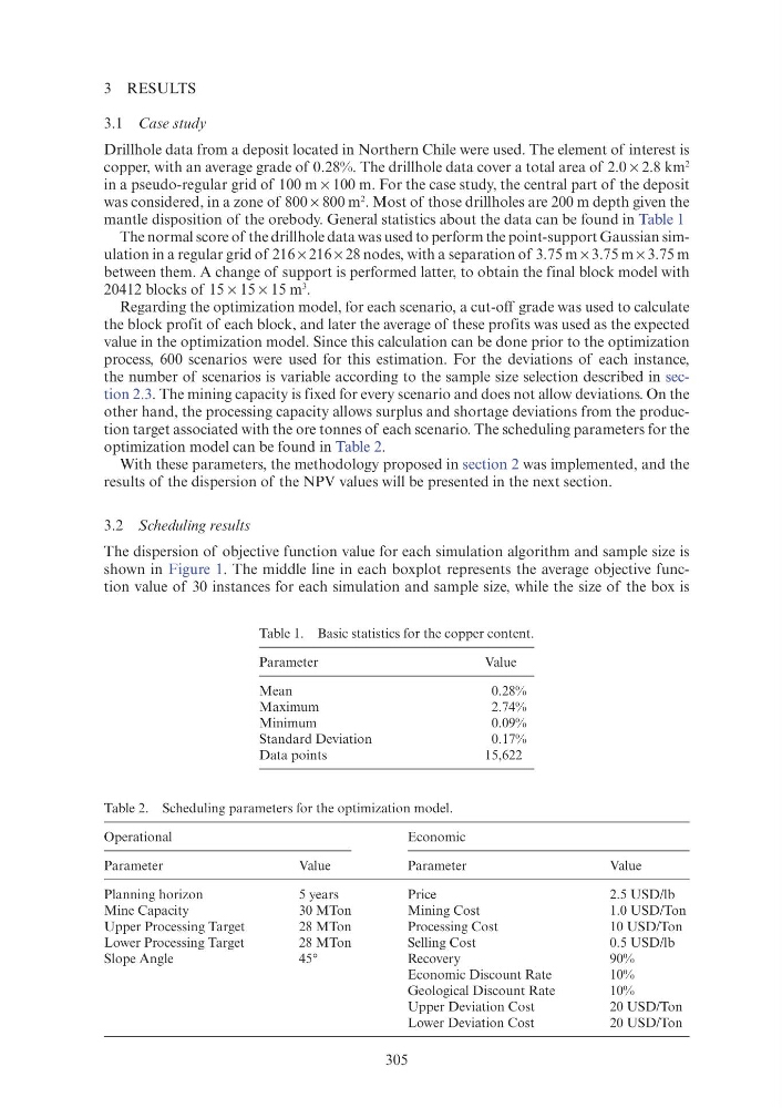
mantle disposition of the orebody. General statistics about the data can be found in Table 1
The normal score of the drillhole data was used to perform the point-support Gaussian simulation in a regular grid of 216 × 216 × 28 nodes, with a separation of 3.75 m × 3.75 m × 3.75 m
between them. A change of support is performed latter, to obtain the final block model with
20412 blocks of 15 × 15 × 15 m
3 .
Regarding the optimization model, for each scenario, a cut-off grade was used to calculate
the block profit of each block, and later the average of these profits was used as the expected
value in the optimization model. Since this calculation can be done prior to the optimization
process, 600 scenarios were used for this estimation. For the deviations of each instance,
the number of scenarios is variable according to the sample size selection described in section 2.3. The mining capacity is fixed for every scenario and does not allow deviations. On the
other hand, the processing capacity allows surplus and shortage deviations from the production target associated with the ore tonnes of each scenario. The scheduling parameters for the
optimization model can be found in Table 2.
With these parameters, the methodology proposed in section 2 was implemented, and the
results of the dispersion of the NPV values will be presented in the next section.
3.2 Scheduling results
The dispersion of objective function value for each simulation algorithm and sample size is
shown in Figure 1. The middle line in each boxplot represents the average objective function value of 30 instances for each simulation and sample size, while the size of the box is
Table 1. Basic statistics for the copper content.
Parameter
Value
Mean
0.28%
Maximum
2.74%
Minimum
0.09%
Standard Deviation
0.17%
Data points
15,622
Table 2. Scheduling parameters for the optimization model.
Operational
Economic
Parameter
Value
Parameter
Value
Planning horizon
5 years
Price
2.5 USD/lb
Mine Capacity
30 MTon
Mining Cost
1.0 USD/Ton
Upper Processing Target
28 MTon
Processing Cost
10 USD/Ton
Lower Processing Target
28 MTon
Selling Cost
0.5 USD/lb
Slope Angle
45°
Recovery
90%
Economic Discount Rate
10%
Geological Discount Rate
10%
Upper Deviation Cost
20 USD/Ton
Lower Deviation Cost
20 USD/Ton
3 RESULTS
3.1 Case study
Drillhole data from a deposit located in Northern Chile were used. The element of interest is
copper, with an average grade of 0.28%. The drillhole data cover a total area of 2.0 × 2.8 km
2
in a pseudo-regular grid of 100 m × 100 m. For the case study, the central part of the deposit
was considered, in a zone of 800 × 800 m
2 . Most of those drillholes are 200 m depth given the
mantle disposition of the orebody. General statistics about the data can be found in Table 1
The normal score of the drillhole data was used to perform the point-support Gaussian simulation in a regular grid of 216 × 216 × 28 nodes, with a separation of 3.75 m × 3.75 m × 3.75 m
between them. A change of support is performed latter, to obtain the final block model with
20412 blocks of 15 × 15 × 15 m
3 .
Regarding the optimization model, for each scenario, a cut-off grade was used to calculate
the block profit of each block, and later the average of these profits was used as the expected
value in the optimization model. Since this calculation can be done prior to the optimization
process, 600 scenarios were used for this estimation. For the deviations of each instance,
the number of scenarios is variable according to the sample size selection described in section 2.3. The mining capacity is fixed for every scenario and does not allow deviations. On the
other hand, the processing capacity allows surplus and shortage deviations from the production target associated with the ore tonnes of each scenario. The scheduling parameters for the
optimization model can be found in Table 2.
With these parameters, the methodology proposed in section 2 was implemented, and the
results of the dispersion of the NPV values will be presented in the next section.
3.2 Scheduling results
The dispersion of objective function value for each simulation algorithm and sample size is
shown in Figure 1. The middle line in each boxplot represents the average objective function value of 30 instances for each simulation and sample size, while the size of the box is
Table 1. Basic statistics for the copper content.
Parameter
Value
Mean
0.28%
Maximum
2.74%
Minimum
0.09%
Standard Deviation
0.17%
Data points
15,622
Table 2. Scheduling parameters for the optimization model.
Operational
Economic
Parameter
Value
Parameter
Value
Planning horizon
5 years
Price
2.5 USD/lb
Mine Capacity
30 MTon
Mining Cost
1.0 USD/Ton
Upper Processing Target
28 MTon
Processing Cost
10 USD/Ton
Lower Processing Target
28 MTon
Selling Cost
0.5 USD/lb
Slope Angle
45°
Recovery
90%
Economic Discount Rate
10%
Geological Discount Rate
10%
Upper Deviation Cost
20 USD/Ton
Lower Deviation Cost
20 USD/Ton