

303
and, simultaneously, maintaining a consistent production target for every scenario. A cut-off
grade is used to classify each block as ore or waste, and since each scenario presents different grades, the same block may have a different classification. Therefore, for the same mine
sequence, some scenarios may have a surplus of ore or metal content from the desired target,
meanwhile others may have a shortage, which are called deviations. Since the excess and
shortage of ore is detrimental for the mining operation, the optimization model incorporates
a cost in the objective function accounting for the deviations from the production targets of
each scenario. Therefore, the model aims to minimize this cost finding a feasible schedule for
all the scenarios at the same time.
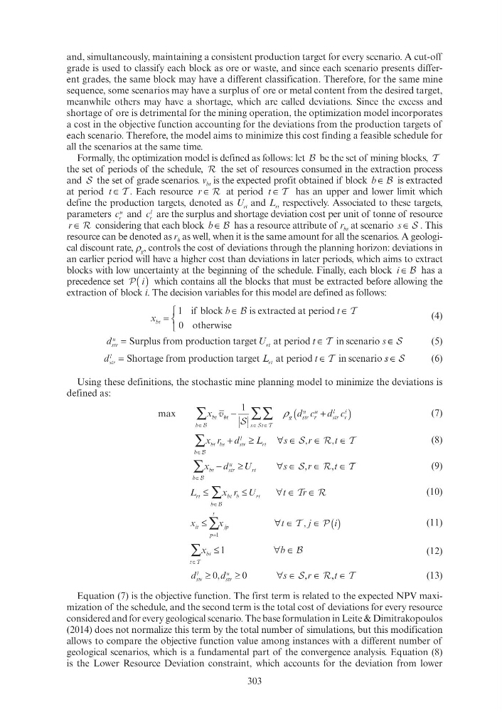
Formally, the optimization model is defined as follows: let B be the set of mining blocks, T
the set of periods of the schedule, R the set of resources consumed in the extraction process
and S the set of grade scenarios. v bt is the expected profit obtained if block b ∈ B is extracted
at period t ∈ T . Each resource r ∈ R at period t ∈ T has an upper and lower limit which
define the production targets, denoted as U rt and L rt respectively. Associated to these targets,
parameters c r
u and c r
l are the surplus and shortage deviation cost per unit of tonne of resource
r ∈ R considering that each block b ∈ B has a resource attribute of r bs at scenario s ∈ S . This
resource can be denoted as r b as well, when it is the same amount for all the scenarios. A geological discount rate, ρ g , controls the cost of deviations through the planning horizon: deviations in
an earlier period will have a higher cost than deviations in later periods, which aims to extract
blocks with low uncertainty at the beginning of the schedule. Finally, each block i ∈ B has a
precedence set P( )
i which contains all the blocks that must be extracted before allowing the
extraction of block i. The decision variables for this model are defined as follows:
x
b
bt =
⎧
⎨
⎧ ⎧
⎩
⎨ ⎨
1
0
if block
i
b
period
otherwise
T
t ∈
t
B is e t acted at period
(4)
d
U
t
s
st
d r
rt
U U
t
rt
U
p
production g
at period
i scenario
T
∈ ∈ S
(5)
d
L
t
st
d r
l
rt
∈
L
t
rt
L
S o tage o production ta get
at period
in scenario
T
s s ∈ S
(6)
Using these definitions, the stochastic mine planning model to minimize the deviations is
defined as:
max
b
t
g
s
g
∈
∈
∑
∑
bt bt
x bt bt
∑ ∑ g (
)
str
u
r
str
l
r
l
s
d c d
r
u
s c
str
u
d s c r
u
B
S
s s
T
S
1
ρ
(7)
b
bt bs
str
l
rt
x r
bt b
d
L
str
l
r
s
t
∈
∑
+ d str
l
∀ ∈
s
∈
t
B
S
R
r ∈
T
,
,
R
r ∈
(8)
b
bt
str
rt
x d
bt
s
U
s
rt
t
∈
∑
≥
str
u
d s
∀ ∈
s
∈
t
B
S
R
r
T
,
,
R
r
(9)
L
x r U
t
rt
L
b
bt b
r
r U
r
t
x r
bt r r
∀ ∈
t
∈
∑ ∑
B
T
R
r ∈
(10)
x
x
t
j
it
p
t
jp
∀
x jp
≤
( )
i
=
∑ x x
∑ x
1
T
P
j ∈
j
(11)
t
bt
x
b
bt
∈
∑
∈
T
B
(12)
d
d
t
st
d r
l
str
∀ ∈
s
∈
t
0
d ≥
d
u
,
s
, str
∀s
0
d st
d r ≥
d st
d r
,
S
R
r ∈
,
T
(13)
Equation (7) is the objective function. The first term is related to the expected NPV maximization of the schedule, and the second term is the total cost of deviations for every resource
considered and for every geological scenario. The base formulation in Leite & Dimitrakopoulos
(2014) does not normalize this term by the total number of simulations, but this modification
allows to compare the objective function value among instances with a different number of
geological scenarios, which is a fundamental part of the convergence analysis. Equation (8)
is the Lower Resource Deviation constraint, which accounts for the deviation from lower
and, simultaneously, maintaining a consistent production target for every scenario. A cut-off
grade is used to classify each block as ore or waste, and since each scenario presents different grades, the same block may have a different classification. Therefore, for the same mine
sequence, some scenarios may have a surplus of ore or metal content from the desired target,
meanwhile others may have a shortage, which are called deviations. Since the excess and
shortage of ore is detrimental for the mining operation, the optimization model incorporates
a cost in the objective function accounting for the deviations from the production targets of
each scenario. Therefore, the model aims to minimize this cost finding a feasible schedule for
all the scenarios at the same time.
Formally, the optimization model is defined as follows: let B be the set of mining blocks, T
the set of periods of the schedule, R the set of resources consumed in the extraction process
and S the set of grade scenarios. v bt is the expected profit obtained if block b ∈ B is extracted
at period t ∈ T . Each resource r ∈ R at period t ∈ T has an upper and lower limit which
define the production targets, denoted as U rt and L rt respectively. Associated to these targets,
parameters c r
u and c r
l are the surplus and shortage deviation cost per unit of tonne of resource
r ∈ R considering that each block b ∈ B has a resource attribute of r bs at scenario s ∈ S . This
resource can be denoted as r b as well, when it is the same amount for all the scenarios. A geological discount rate, ρ g , controls the cost of deviations through the planning horizon: deviations in
an earlier period will have a higher cost than deviations in later periods, which aims to extract
blocks with low uncertainty at the beginning of the schedule. Finally, each block i ∈ B has a
precedence set P( )
i which contains all the blocks that must be extracted before allowing the
extraction of block i. The decision variables for this model are defined as follows:
x
b
bt =
⎧
⎨
⎧ ⎧
⎩
⎨ ⎨
1
0
if block
i
b
period
otherwise
T
t ∈
t
B is e t acted at period
(4)
d
U
t
s
st
d r
rt
U U
t
rt
U
p
production g
at period
i scenario
T
∈ ∈ S
(5)
d
L
t
st
d r
l
rt
∈
L
t
rt
L
S o tage o production ta get
at period
in scenario
T
s s ∈ S
(6)
Using these definitions, the stochastic mine planning model to minimize the deviations is
defined as:
max
b
t
g
s
g
∈
∈
∑
∑
bt bt
x bt bt
∑ ∑ g (
)
str
u
r
str
l
r
l
s
d c d
r
u
s c
str
u
d s c r
u
B
S
s s
T
S
1
ρ
(7)
b
bt bs
str
l
rt
x r
bt b
d
L
str
l
r
s
t
∈
∑
+ d str
l
∀ ∈
s
∈
t
B
S
R
r ∈
T
,
,
R
r ∈
(8)
b
bt
str
rt
x d
bt
s
U
s
rt
t
∈
∑
≥
str
u
d s
∀ ∈
s
∈
t
B
S
R
r
T
,
,
R
r
(9)
L
x r U
t
rt
L
b
bt b
r
r U
r
t
x r
bt r r
∀ ∈
t
∈
∑ ∑
B
T
R
r ∈
(10)
x
x
t
j
it
p
t
jp
∀
x jp
≤
( )
i
=
∑ x x
∑ x
1
T
P
j ∈
j
(11)
t
bt
x
b
bt
∈
∑
∈
T
B
(12)
d
d
t
st
d r
l
str
∀ ∈
s
∈
t
0
d ≥
d
u
,
s
, str
∀s
0
d st
d r ≥
d st
d r
,
S
R
r ∈
,
T
(13)
Equation (7) is the objective function. The first term is related to the expected NPV maximization of the schedule, and the second term is the total cost of deviations for every resource
considered and for every geological scenario. The base formulation in Leite & Dimitrakopoulos
(2014) does not normalize this term by the total number of simulations, but this modification
allows to compare the objective function value among instances with a different number of
geological scenarios, which is a fundamental part of the convergence analysis. Equation (8)
is the Lower Resource Deviation constraint, which accounts for the deviation from lower