

302
scenarios, and the random numbers for each node are drawn beforehand. Moreover, a correlation matrix is imposed to these random numbers to obtain a negative pairwise correlation
among every scenario. Then, the negative correlation of the random number transfers to the
complete simulated scenarios.
Formally, let m be the number of simulated scenarios required, and n the number of nodes
in each scenario. To simulate these m scenarios, m standard Gaussian vectors of size n are
needed, one vector for each scenario and one element of these vectors for each node. To
achieve the negative correlation between scenarios, a correlation matrix is imposed to these m
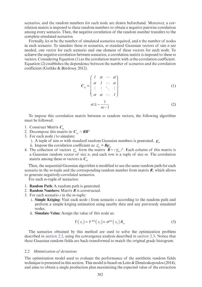
vectors. Considering Equation (1) as the correlation matrix with α the correlation coefficient.
Equation (2) establishes the dependence between the number of scenarios and the correlation
coefficient (Guthke & Bárdossy 2012).
C m =
1
1
1
α
α
α
α
1
α α
⎛
⎝
⎜
⎛ ⎛
⎜
⎜ ⎜
⎜
⎜ ⎜
⎜ ⎝ ⎝
⎜ ⎜
⎞
⎠
⎟
⎞ ⎞
⎟
⎟ ⎟
⎟
⎟ ⎟
⎟ ⎠ ⎠
⎟ ⎟
(1)
α ≥ − −
1
1
m
(2)
To impose this correlation matrix between m random vectors, the following algorithm
must be followed:
1. Construct Matrix C m
2. Decompose this matrix in C
BB
m
T
3. For each node i to simulate:
i. A tuple of size m with standard random Gaussian numbers is generated, g m
i
ii. Impose the correlation coefficient as z
Bg
B
m
i
m
i
4. The collection of vectors z m
i form the matrix R ( )
z
.
m
i T
) Each column of this matrix is
a Gaussian random vector of size n, and each row is a tuple of size m. The correlation
matrix among these m vectors is C m
Then, the sequential Gaussian algorithm is modified to use the same random path for each
scenario in the m-tuple and the corresponding random number from matrix R, which allows
to generate negatively-correlated scenarios.
For each m-tuple of scenarios:
1. Random Path: A random path is generated.
2. Random Numbers: Matrix R is constructed.
3. For each scenario s in the m-tuple:
i. Simple Kriging: Visit each node i from scenario s according to the random path and
perform a simple kriging estimation using nearby data and any previously simulated
nodes.
ii. Simulate Value: Assign the value of this node as:
Y
Y
R
KS
KS
i
R ,s
i
( )
x i =
( )
x i +
( )
x i
σ
K K
(3)
The scenarios obtained by this method are used to solve the optimization problem
described in section 2.2, using the convergence analysis described in section 2.3. Notice that
these Gaussian random fields are back-transformed to match the original grade histogram.
2.2 Minimization of deviations
The optimization model used to evaluate the performance of the antithetic random fields
technique is presented in this section. This model is based on Leite & Dimitrakopoulos (2014),
and aims to obtain a single production plan maximizing the expected value of the extraction
scenarios, and the random numbers for each node are drawn beforehand. Moreover, a correlation matrix is imposed to these random numbers to obtain a negative pairwise correlation
among every scenario. Then, the negative correlation of the random number transfers to the
complete simulated scenarios.
Formally, let m be the number of simulated scenarios required, and n the number of nodes
in each scenario. To simulate these m scenarios, m standard Gaussian vectors of size n are
needed, one vector for each scenario and one element of these vectors for each node. To
achieve the negative correlation between scenarios, a correlation matrix is imposed to these m
vectors. Considering Equation (1) as the correlation matrix with α the correlation coefficient.
Equation (2) establishes the dependence between the number of scenarios and the correlation
coefficient (Guthke & Bárdossy 2012).
C m =
1
1
1
α
α
α
α
1
α α
⎛
⎝
⎜
⎛ ⎛
⎜
⎜ ⎜
⎜
⎜ ⎜
⎜ ⎝ ⎝
⎜ ⎜
⎞
⎠
⎟
⎞ ⎞
⎟
⎟ ⎟
⎟
⎟ ⎟
⎟ ⎠ ⎠
⎟ ⎟
(1)
α ≥ − −
1
1
m
(2)
To impose this correlation matrix between m random vectors, the following algorithm
must be followed:
1. Construct Matrix C m
2. Decompose this matrix in C
BB
m
T
3. For each node i to simulate:
i. A tuple of size m with standard random Gaussian numbers is generated, g m
i
ii. Impose the correlation coefficient as z
Bg
B
m
i
m
i
4. The collection of vectors z m
i form the matrix R ( )
z
.
m
i T
) Each column of this matrix is
a Gaussian random vector of size n, and each row is a tuple of size m. The correlation
matrix among these m vectors is C m
Then, the sequential Gaussian algorithm is modified to use the same random path for each
scenario in the m-tuple and the corresponding random number from matrix R, which allows
to generate negatively-correlated scenarios.
For each m-tuple of scenarios:
1. Random Path: A random path is generated.
2. Random Numbers: Matrix R is constructed.
3. For each scenario s in the m-tuple:
i. Simple Kriging: Visit each node i from scenario s according to the random path and
perform a simple kriging estimation using nearby data and any previously simulated
nodes.
ii. Simulate Value: Assign the value of this node as:
Y
Y
R
KS
KS
i
R ,s
i
( )
x i =
( )
x i +
( )
x i
σ
K K
(3)
The scenarios obtained by this method are used to solve the optimization problem
described in section 2.2, using the convergence analysis described in section 2.3. Notice that
these Gaussian random fields are back-transformed to match the original grade histogram.
2.2 Minimization of deviations
The optimization model used to evaluate the performance of the antithetic random fields
technique is presented in this section. This model is based on Leite & Dimitrakopoulos (2014),
and aims to obtain a single production plan maximizing the expected value of the extraction