

187
As a test, the stratigraphic correction for the footwall, hangwall and average of the mineralized layer was carried out and the variography and cross validation using ordinary kriging
of them were made in opposition to the real coordinates. The stratigraphic correction by the
hangwall of the layer was adopted because it presented the smallest variance of the error
obtained by cross validation.
3.3 Variogram analysis and modeling
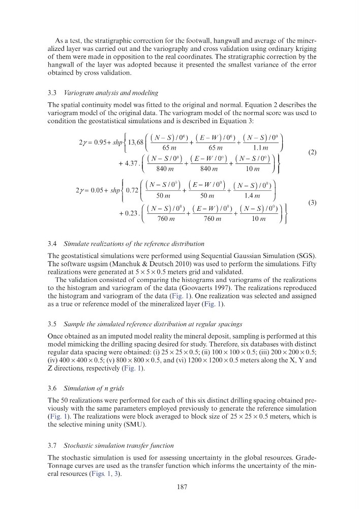
The spatial continuity model was fitted to the original and normal. Equation 2 describes the
variogram model of the original data. The variogram model of the normal score was used to
condition the geostatistical simulations and is described in Equation 3:
2
095
13 68
65
65
0
1 1
0
0
0
γ
+
0 95
(
)
+
(
)
+
(
)
⎛
⎝ ⎜
⎛ ⎛
⎝ ⎝
⎞
.
,
95
13
+
95
/ )
0
0
/ )
0
0
0
/
.
shp h
−
m
−
m
−
m
⎠ ⎠ ⎟
⎞ ⎞
⎠ ⎠ ⎠ ⎠
⎧
⎨
⎧ ⎧
⎨ ⎨
⎧ ⎧ ⎧ ⎧
⎩ ⎩ ⎩
⎨ ⎨ ⎨ ⎨
+
(
) + (
) + (
)
⎛
⎝ ⎜
⎛ ⎛
⎝ ⎝
⎞
⎠ ⎟
⎞ ⎞
⎠ ⎠
⎫
4 37
840
840
10
) (
. .
37
) (
) (
−
m
−
m
−
m
⎬ ⎬
⎫ ⎫
⎬ ⎬ ⎬ ⎬
⎫ ⎫ ⎫ ⎫ ⎫ ⎫ ⎫
⎭
⎬ ⎬ ⎬ ⎬
⎭ ⎭
⎬ ⎬ ⎬ ⎬ ⎬ ⎬ ⎬
(2)
2
005
0 72
50
0
50
1 4
0
0
0
0
γ
+
0 05
(
) + (
) + (
)
⎛
⎝
⎜
⎛ ⎛
⎝ ⎝
⎞
⎠
⎟
⎞ ⎞
⎠ ⎠
.
0
.05 +
05
/
/
0
0
) (
/ )
0
0
.
shp h
N S
−
m
−
m
−
m
⎧ ⎧
⎨
⎪ ⎧ ⎧ ⎧ ⎧
⎨ ⎨
⎩ ⎪
⎨ ⎨
⎩ ⎩
+
(
)
+
(
)
+
(
)
⎛
⎝ ⎜
⎛ ⎛
⎝ ⎝
⎞
⎠ ⎟
⎞ ⎞
⎠ ⎠
0 23
760
760
10
0
0
(
)
0
. .
23
/ )
0
0
/ )
0
0
0
/ )
0
0
−
m
−
m
−
m
⎫ ⎫
⎬
⎫ ⎫ ⎫ ⎫
⎬ ⎬
⎫ ⎫ ⎫ ⎫ ⎫ ⎫ ⎫
⎭
⎬ ⎬
⎭ ⎭
⎬ ⎬ ⎬ ⎬
(3)
3.4 Simulate realizations of the reference distribution
The geostatistical simulations were performed using Sequential Gaussian Simulation (SGS).
The software usgsim (Manchuk & Deutsch 2010) was used to perform the simulations. Fifty
realizations were generated at 5 × 5 × 0.5 meters grid and validated.
The validation consisted of comparing the histograms and variograms of the realizations
to the histogram and variogram of the data (Goovaerts 1997). The realizations reproduced
the histogram and variogram of the data (Fig. 1). One realization was selected and assigned
as a true or reference model of the mineralized layer (Fig. 1).
3.5 Sample the simulated reference distribution at regular spacings
Once obtained as an imputed model reality the mineral deposit, sampling is performed at this
model mimicking the drilling spacing desired for study. Therefore, six databases with distinct
regular data spacing were obtained: (i) 25 × 25 × 0.5; (ii) 100 × 100 × 0.5; (iii) 200 × 200 × 0.5;
(iv) 400 × 400 × 0.5; (v) 800 × 800 × 0.5, and (vi) 1200 × 1200 × 0.5 meters along the X, Y and
Z directions, respectively (Fig. 1).
3.6 Simulation of n grids
The 50 realizations were performed for each of this six distinct drilling spacing obtained previously with the same parameters employed previously to generate the reference simulation
(Fig. 1). The realizations were block averaged to block size of 25 × 25 × 0.5 meters, which is
the selective mining unity (SMU).
3.7 Stochastic simulation transfer function
The stochastic simulation is used for assessing uncertainty in the global resources. GradeTonnage curves are used as the transfer function which informs the uncertainty of the mineral resources (Figs. 1, 3).
As a test, the stratigraphic correction for the footwall, hangwall and average of the mineralized layer was carried out and the variography and cross validation using ordinary kriging
of them were made in opposition to the real coordinates. The stratigraphic correction by the
hangwall of the layer was adopted because it presented the smallest variance of the error
obtained by cross validation.
3.3 Variogram analysis and modeling
The spatial continuity model was fitted to the original and normal. Equation 2 describes the
variogram model of the original data. The variogram model of the normal score was used to
condition the geostatistical simulations and is described in Equation 3:
2
095
13 68
65
65
0
1 1
0
0
0
γ
+
0 95
(
)
+
(
)
+
(
)
⎛
⎝ ⎜
⎛ ⎛
⎝ ⎝
⎞
.
,
95
13
+
95
/ )
0
0
/ )
0
0
0
/
.
shp h
−
m
−
m
−
m
⎠ ⎠ ⎟
⎞ ⎞
⎠ ⎠ ⎠ ⎠
⎧
⎨
⎧ ⎧
⎨ ⎨
⎧ ⎧ ⎧ ⎧
⎩ ⎩ ⎩
⎨ ⎨ ⎨ ⎨
+
(
) + (
) + (
)
⎛
⎝ ⎜
⎛ ⎛
⎝ ⎝
⎞
⎠ ⎟
⎞ ⎞
⎠ ⎠
⎫
4 37
840
840
10
) (
. .
37
) (
) (
−
m
−
m
−
m
⎬ ⎬
⎫ ⎫
⎬ ⎬ ⎬ ⎬
⎫ ⎫ ⎫ ⎫ ⎫ ⎫ ⎫
⎭
⎬ ⎬ ⎬ ⎬
⎭ ⎭
⎬ ⎬ ⎬ ⎬ ⎬ ⎬ ⎬
(2)
2
005
0 72
50
0
50
1 4
0
0
0
0
γ
+
0 05
(
) + (
) + (
)
⎛
⎝
⎜
⎛ ⎛
⎝ ⎝
⎞
⎠
⎟
⎞ ⎞
⎠ ⎠
.
0
.05 +
05
/
/
0
0
) (
/ )
0
0
.
shp h
N S
−
m
−
m
−
m
⎧ ⎧
⎨
⎪ ⎧ ⎧ ⎧ ⎧
⎨ ⎨
⎩ ⎪
⎨ ⎨
⎩ ⎩
+
(
)
+
(
)
+
(
)
⎛
⎝ ⎜
⎛ ⎛
⎝ ⎝
⎞
⎠ ⎟
⎞ ⎞
⎠ ⎠
0 23
760
760
10
0
0
(
)
0
. .
23
/ )
0
0
/ )
0
0
0
/ )
0
0
−
m
−
m
−
m
⎫ ⎫
⎬
⎫ ⎫ ⎫ ⎫
⎬ ⎬
⎫ ⎫ ⎫ ⎫ ⎫ ⎫ ⎫
⎭
⎬ ⎬
⎭ ⎭
⎬ ⎬ ⎬ ⎬
(3)
3.4 Simulate realizations of the reference distribution
The geostatistical simulations were performed using Sequential Gaussian Simulation (SGS).
The software usgsim (Manchuk & Deutsch 2010) was used to perform the simulations. Fifty
realizations were generated at 5 × 5 × 0.5 meters grid and validated.
The validation consisted of comparing the histograms and variograms of the realizations
to the histogram and variogram of the data (Goovaerts 1997). The realizations reproduced
the histogram and variogram of the data (Fig. 1). One realization was selected and assigned
as a true or reference model of the mineralized layer (Fig. 1).
3.5 Sample the simulated reference distribution at regular spacings
Once obtained as an imputed model reality the mineral deposit, sampling is performed at this
model mimicking the drilling spacing desired for study. Therefore, six databases with distinct
regular data spacing were obtained: (i) 25 × 25 × 0.5; (ii) 100 × 100 × 0.5; (iii) 200 × 200 × 0.5;
(iv) 400 × 400 × 0.5; (v) 800 × 800 × 0.5, and (vi) 1200 × 1200 × 0.5 meters along the X, Y and
Z directions, respectively (Fig. 1).
3.6 Simulation of n grids
The 50 realizations were performed for each of this six distinct drilling spacing obtained previously with the same parameters employed previously to generate the reference simulation
(Fig. 1). The realizations were block averaged to block size of 25 × 25 × 0.5 meters, which is
the selective mining unity (SMU).
3.7 Stochastic simulation transfer function
The stochastic simulation is used for assessing uncertainty in the global resources. GradeTonnage curves are used as the transfer function which informs the uncertainty of the mineral resources (Figs. 1, 3).