

186
6. Geostatistical Simulation using the n databases with regular spacing;
7. Calculation of grade-tonnage curves for all the realizations;
8. Summarize uncertainty measures.
3.1 Exploratory data analysis
This case study uses a database of a large mine in one of the greatest bauxite plateaus of the
Brazilian Amazon. The data cover approximately an irregular area of 10 km on the east-west
axis and 4.5 km on the north-south axis. There are 4 drilling grids: 200 × 200, 100 × 100,
50 × 50 and 25 × 25 meters along the X and Y directions.
The bauxite mineralization is formed by lateritic processes typical of tropical zones and
started in the early Cenozoic age, acting over immature sandstones and mudstones forming
extensive layers at kilometric plateau formations. The capping of non-mineralized clay varies
from 0.5 to 12 meters.
One main seam of bauxite ore in the database was chosen for the case study. This mineralized seam has an average thickness of 1,5 meters. Furthermore, this seam contains 2784 drill
holes with 7609 geochemical samples at an average length of 0.5 meters.
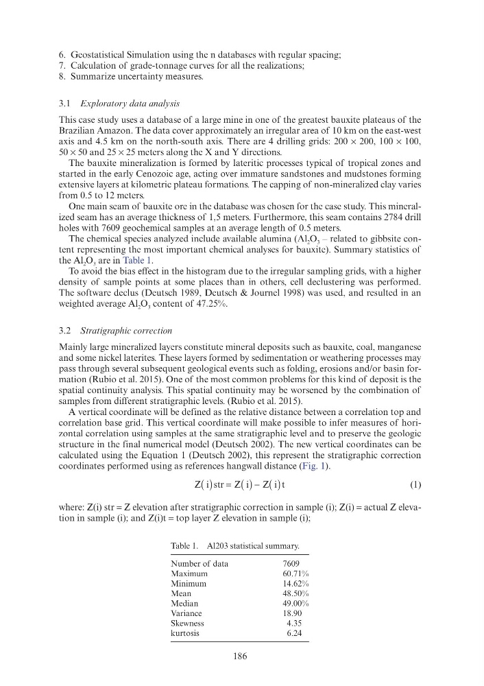
The chemical species analyzed include available alumina (Al 2 O 3 – related to gibbsite content representing the most important chemical analyses for bauxite). Summary statistics of
the Al 2 O 3 are in Table 1.
To avoid the bias effect in the histogram due to the irregular sampling grids, with a higher
density of sample points at some places than in others, cell declustering was performed.
The software declus (Deutsch 1989, Deutsch & Journel 1998) was used, and resulted in an
weighted average Al 2 O 3 content of 47.25%.
3.2 Stratigraphic correction
Mainly large mineralized layers constitute mineral deposits such as bauxite, coal, manganese
and some nickel laterites. These layers formed by sedimentation or weathering processes may
pass through several subsequent geological events such as folding, erosions and/or basin formation (Rubio et al. 2015). One of the most common problems for this kind of deposit is the
spatial continuity analysis. This spatial continuity may be worsened by the combination of
samples from different stratigraphic levels. (Rubio et al. 2015).
A vertical coordinate will be defined as the relative distance between a correlation top and
correlation base grid. This vertical coordinate will make possible to infer measures of horizontal correlation using samples at the same stratigraphic level and to preserve the geologic
structure in the final numerical model (Deutsch 2002). The new vertical coordinates can be
calculated using the Equation 1 (Deutsch 2002), this represent the stratigraphic correction
coordinates performed using as references hangwall distance (Fig. 1).
Z str Z
Z t
( )
i
( )
i
( )
i
(1)
where: Z(i) str = Z elevation after stratigraphic correction in sample (i); Z(i) = actual Z elevation in sample (i); and Z(i)t = top layer Z elevation in sample (i);
Table 1. Al203 statistical summary.
Number of data
7609
Maximum
60.71%
Minimum
14.62%
Mean
48.50%
Median
49.00%
Variance
18.90
Skewness
4.35
kurtosis
6.24
6. Geostatistical Simulation using the n databases with regular spacing;
7. Calculation of grade-tonnage curves for all the realizations;
8. Summarize uncertainty measures.
3.1 Exploratory data analysis
This case study uses a database of a large mine in one of the greatest bauxite plateaus of the
Brazilian Amazon. The data cover approximately an irregular area of 10 km on the east-west
axis and 4.5 km on the north-south axis. There are 4 drilling grids: 200 × 200, 100 × 100,
50 × 50 and 25 × 25 meters along the X and Y directions.
The bauxite mineralization is formed by lateritic processes typical of tropical zones and
started in the early Cenozoic age, acting over immature sandstones and mudstones forming
extensive layers at kilometric plateau formations. The capping of non-mineralized clay varies
from 0.5 to 12 meters.
One main seam of bauxite ore in the database was chosen for the case study. This mineralized seam has an average thickness of 1,5 meters. Furthermore, this seam contains 2784 drill
holes with 7609 geochemical samples at an average length of 0.5 meters.
The chemical species analyzed include available alumina (Al 2 O 3 – related to gibbsite content representing the most important chemical analyses for bauxite). Summary statistics of
the Al 2 O 3 are in Table 1.
To avoid the bias effect in the histogram due to the irregular sampling grids, with a higher
density of sample points at some places than in others, cell declustering was performed.
The software declus (Deutsch 1989, Deutsch & Journel 1998) was used, and resulted in an
weighted average Al 2 O 3 content of 47.25%.
3.2 Stratigraphic correction
Mainly large mineralized layers constitute mineral deposits such as bauxite, coal, manganese
and some nickel laterites. These layers formed by sedimentation or weathering processes may
pass through several subsequent geological events such as folding, erosions and/or basin formation (Rubio et al. 2015). One of the most common problems for this kind of deposit is the
spatial continuity analysis. This spatial continuity may be worsened by the combination of
samples from different stratigraphic levels. (Rubio et al. 2015).
A vertical coordinate will be defined as the relative distance between a correlation top and
correlation base grid. This vertical coordinate will make possible to infer measures of horizontal correlation using samples at the same stratigraphic level and to preserve the geologic
structure in the final numerical model (Deutsch 2002). The new vertical coordinates can be
calculated using the Equation 1 (Deutsch 2002), this represent the stratigraphic correction
coordinates performed using as references hangwall distance (Fig. 1).
Z str Z
Z t
( )
i
( )
i
( )
i
(1)
where: Z(i) str = Z elevation after stratigraphic correction in sample (i); Z(i) = actual Z elevation in sample (i); and Z(i)t = top layer Z elevation in sample (i);
Table 1. Al203 statistical summary.
Number of data
7609
Maximum
60.71%
Minimum
14.62%
Mean
48.50%
Median
49.00%
Variance
18.90
Skewness
4.35
kurtosis
6.24