

164
Cov
Cov
C C
Cov
C ov
C C
Au
Au Cu
Cu Au
Cu
/
/
.
.
.
.
⎛
⎝ ⎜
⎛ ⎛
⎝ ⎝
⎞
⎠ ⎟
⎞ ⎞
⎠ ⎠
=
−
−
⎛
⎝ ⎜
⎛ ⎛
⎝ ⎝
⎞
⎠ ⎟
⎞ ⎞
⎠ ⎠
15 37
1 0
. 6
1 0
. 6 0 07
nugge n n
t
S ph
S
⎛
⎝ ⎝ ⎝
⎞
⎠ ⎠ ⎠
(
)
m
m
m
39 24 5 14
5 14 0 67
.
.
24 5
.
.
14 0
m m
(5)
Positive semi-definite condition of the sill matrix was also examined. This implies that
the fitted linear model of coregionalization is mathematically sound and the direct and
cross-covariances can be used for establishing the ordinary multi-collocated cokriging system. To do so, the same moving neighborhood characterization as it was used for estimation of the copper grade, is considered in this case. A neighborhood with conditioning up
to 100 surrounding data characterized by radiuses equal to 200 m, derived from the direct
and cross-covariances. In order to make a comparison, a unique neighborhood in ordinary
multi-collocated cokriging system is also considered for benchmarking. In this cokriging
paradigm, which is theoretically sound, one uses all the conditioning data for estimation
process, for which it does not lead to a loss of accuracy that may happen in moving neighborhood (Emery, 2004). However, the computation restrictions is one reason to switching from
unique to moving neighborhood in usual co-estimation workflows. Conventional cokriging
system also is taken into account for further testing the algorithm. To do so, an isotopic
searching strategy is opted, in which 100 closest sampling points containing both the primary
and secondary variables are attended in a moving neighborhood. This practice is indeed typical in block modeling for mineral resource estimation in mining industry.
Figure 6 illustrates the produced maps for the target variable, gold and also secondary variable, copper. In all the maps, the results of estimated gold grades in ordinary multi-collocated
cokriging for the case of moving neighborhood bear relatively resemblance to the case of
ordinary multi-collocated cokriging with unique neighborhood. In copper grade, however
the results are exactly the same in two underlying maps, because two methods use the same
estimated copper grade values as secondary information which already was produced through
step 1 by ordinary kriging. The outputs for traditional ordinary cokriging system with isotopic
searching strategy is, however somehow different in some areas. For instance, in coordinate
(East: 200 m and North: 450 m), the latter approach is failed to estimate the high values of gold
and copper grade. Nevertheless, the smoothing effect in all the cases show the same outcome
due to (co)-kriging assumptions. Another examination over the three methodologies relates to
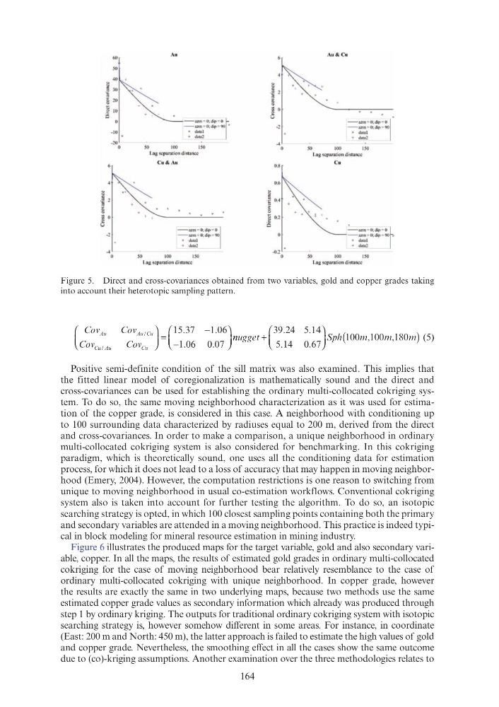
Figure 5. Direct and cross-covariances obtained from two variables, gold and copper grades taking
into account their heterotopic sampling pattern.
60
Au
50
40
g
c;
-~m - o,o;p - o I'
-
nzm = O;dip = 9tl ~
-10
w dtlal
+ d:tlu2
-20
0
so
100
150
Lag separation distance
Cu&Au
g
·~ 2
~
~
0
-~m · O, dlp • O I
-2
-
azm = O:dip = 'JO
~
du;~l
+ datal
_
-4
0
50
100
150
Lag separation distance
'
~
u
0
-2
-4
0
0.8
-~ 0.4
~
8
2
02
c;
-0.2
()
50
so
Au& Cu
100
-~m · O,dlp • O I
-
;'l%m =O:dip :90
~
d;tl
ISO
Lag separation d ista nce
Cu
':__~m:"'"':" r
-
nzm - O.dlp -90 x
~
d;ua l
+ d;lla2
100
150
Lag separation d istance
Cov
Cov
C C
Cov
C ov
C C
Au
Au Cu
Cu Au
Cu
/
/
.
.
.
.
⎛
⎝ ⎜
⎛ ⎛
⎝ ⎝
⎞
⎠ ⎟
⎞ ⎞
⎠ ⎠
=
−
−
⎛
⎝ ⎜
⎛ ⎛
⎝ ⎝
⎞
⎠ ⎟
⎞ ⎞
⎠ ⎠
15 37
1 0
. 6
1 0
. 6 0 07
nugge n n
t
S ph
S
⎛
⎝ ⎝ ⎝
⎞
⎠ ⎠ ⎠
(
)
m
m
m
39 24 5 14
5 14 0 67
.
.
24 5
.
.
14 0
m m
(5)
Positive semi-definite condition of the sill matrix was also examined. This implies that
the fitted linear model of coregionalization is mathematically sound and the direct and
cross-covariances can be used for establishing the ordinary multi-collocated cokriging system. To do so, the same moving neighborhood characterization as it was used for estimation of the copper grade, is considered in this case. A neighborhood with conditioning up
to 100 surrounding data characterized by radiuses equal to 200 m, derived from the direct
and cross-covariances. In order to make a comparison, a unique neighborhood in ordinary
multi-collocated cokriging system is also considered for benchmarking. In this cokriging
paradigm, which is theoretically sound, one uses all the conditioning data for estimation
process, for which it does not lead to a loss of accuracy that may happen in moving neighborhood (Emery, 2004). However, the computation restrictions is one reason to switching from
unique to moving neighborhood in usual co-estimation workflows. Conventional cokriging
system also is taken into account for further testing the algorithm. To do so, an isotopic
searching strategy is opted, in which 100 closest sampling points containing both the primary
and secondary variables are attended in a moving neighborhood. This practice is indeed typical in block modeling for mineral resource estimation in mining industry.
Figure 6 illustrates the produced maps for the target variable, gold and also secondary variable, copper. In all the maps, the results of estimated gold grades in ordinary multi-collocated
cokriging for the case of moving neighborhood bear relatively resemblance to the case of
ordinary multi-collocated cokriging with unique neighborhood. In copper grade, however
the results are exactly the same in two underlying maps, because two methods use the same
estimated copper grade values as secondary information which already was produced through
step 1 by ordinary kriging. The outputs for traditional ordinary cokriging system with isotopic
searching strategy is, however somehow different in some areas. For instance, in coordinate
(East: 200 m and North: 450 m), the latter approach is failed to estimate the high values of gold
and copper grade. Nevertheless, the smoothing effect in all the cases show the same outcome
due to (co)-kriging assumptions. Another examination over the three methodologies relates to
Figure 5. Direct and cross-covariances obtained from two variables, gold and copper grades taking
into account their heterotopic sampling pattern.
60
Au
50
40
g
c;
-~m - o,o;p - o I'
-
nzm = O;dip = 9tl ~
-10
w dtlal
+ d:tlu2
-20
0
so
100
150
Lag separation distance
Cu&Au
g
·~ 2
~
~
0
-~m · O, dlp • O I
-2
-
azm = O:dip = 'JO
~
du;~l
+ datal
_
-4
0
50
100
150
Lag separation distance
'
~
u
0
-2
-4
0
0.8
-~ 0.4
~
8
2
02
c;
-0.2
()
50
so
Au& Cu
100
-~m · O,dlp • O I
-
;'l%m =O:dip :90
~
d;tl
ISO
Lag separation d ista nce
Cu
':__~m:"'"':" r
-
nzm - O.dlp -90 x
~
d;ua l
+ d;lla2
100
150
Lag separation d istance