

132
Gaussian Simulation (Fig. 7b) in the minor and major directions. The results showed that the
spatial continuity was reproduced in both methodologies.
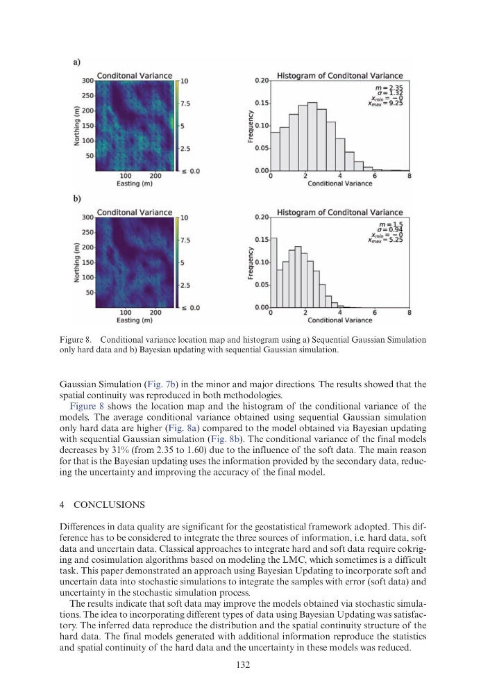
Figure 8 shows the location map and the histogram of the conditional variance of the
models. The average conditional variance obtained using sequential Gaussian simulation
only hard data are higher (Fig. 8a) compared to the model obtained via Bayesian updating
with sequential Gaussian simulation (Fig. 8b). The conditional variance of the final models
decreases by 31% (from 2.35 to 1.60) due to the influence of the soft data. The main reason
for that is the Bayesian updating uses the information provided by the secondary data, reducing the uncertainty and improving the accuracy of the final model.
4 CONCLUSIONS
Differences in data quality are significant for the geostatistical framework adopted. This difference has to be considered to integrate the three sources of information, i.e. hard data, soft
data and uncertain data. Classical approaches to integrate hard and soft data require cokriging and cosimulation algorithms based on modeling the LMC, which sometimes is a difficult
task. This paper demonstrated an approach using Bayesian Updating to incorporate soft and
uncertain data into stochastic simulations to integrate the samples with error (soft data) and
uncertainty in the stochastic simulation process.
The results indicate that soft data may improve the models obtained via stochastic simulations. The idea to incorporating different types of data using Bayesian Updating was satisfactory. The inferred data reproduce the distribution and the spatial continuity structure of the
hard data. The final models generated with additional information reproduce the statistics
and spatial continuity of the hard data and the uncertainty in these models was reduced.
Figure 8. Conditional variance location map and histogram using a) Sequential Gaussian Simulation
only hard data and b) Bayesian updating with sequential Gaussian simulation.
a)
300 Conditonal Variance 10
7.5
Cl
c
5
:c
t:'
0
z
2.5
s 0.0
Easting (m)
b)
300 Conditonal Variance 10
7.5
Cl
c
5
:c
t:'
0
z
2.5
100
200
s 0.0
Easting (m)
>u
c
0.20
0.15
~ 0.10
Histogram of Conditonal Variance
m=2.35
a= 1.32
Xmin = - 0
_ -
Xmax = 9.25
-
rr
-
~
u..
>u
c
0.05
0.00 0
0.20
0.15
~ 0.10
rr
~
u..
0.05
0.00 0
-
~
2
4
6
Conditional Variance
Histogram of Conditonal Variance
m= 1.5
a=0 .94
Xmin = -0
X max = 5 .25
1h
2
4
6
Condit ional Variance
8
8
Gaussian Simulation (Fig. 7b) in the minor and major directions. The results showed that the
spatial continuity was reproduced in both methodologies.
Figure 8 shows the location map and the histogram of the conditional variance of the
models. The average conditional variance obtained using sequential Gaussian simulation
only hard data are higher (Fig. 8a) compared to the model obtained via Bayesian updating
with sequential Gaussian simulation (Fig. 8b). The conditional variance of the final models
decreases by 31% (from 2.35 to 1.60) due to the influence of the soft data. The main reason
for that is the Bayesian updating uses the information provided by the secondary data, reducing the uncertainty and improving the accuracy of the final model.
4 CONCLUSIONS
Differences in data quality are significant for the geostatistical framework adopted. This difference has to be considered to integrate the three sources of information, i.e. hard data, soft
data and uncertain data. Classical approaches to integrate hard and soft data require cokriging and cosimulation algorithms based on modeling the LMC, which sometimes is a difficult
task. This paper demonstrated an approach using Bayesian Updating to incorporate soft and
uncertain data into stochastic simulations to integrate the samples with error (soft data) and
uncertainty in the stochastic simulation process.
The results indicate that soft data may improve the models obtained via stochastic simulations. The idea to incorporating different types of data using Bayesian Updating was satisfactory. The inferred data reproduce the distribution and the spatial continuity structure of the
hard data. The final models generated with additional information reproduce the statistics
and spatial continuity of the hard data and the uncertainty in these models was reduced.
Figure 8. Conditional variance location map and histogram using a) Sequential Gaussian Simulation
only hard data and b) Bayesian updating with sequential Gaussian simulation.
a)
300 Conditonal Variance 10
7.5
Cl
c
5
:c
t:'
0
z
2.5
s 0.0
Easting (m)
b)
300 Conditonal Variance 10
7.5
Cl
c
5
:c
t:'
0
z
2.5
100
200
s 0.0
Easting (m)
>u
c
0.20
0.15
~ 0.10
Histogram of Conditonal Variance
m=2.35
a= 1.32
Xmin = - 0
_ -
Xmax = 9.25
-
rr
-
~
u..
>u
c
0.05
0.00 0
0.20
0.15
~ 0.10
rr
~
u..
0.05
0.00 0
-
~
2
4
6
Conditional Variance
Histogram of Conditonal Variance
m= 1.5
a=0 .94
Xmin = -0
X max = 5 .25
1h
2
4
6
Condit ional Variance
8
8