131
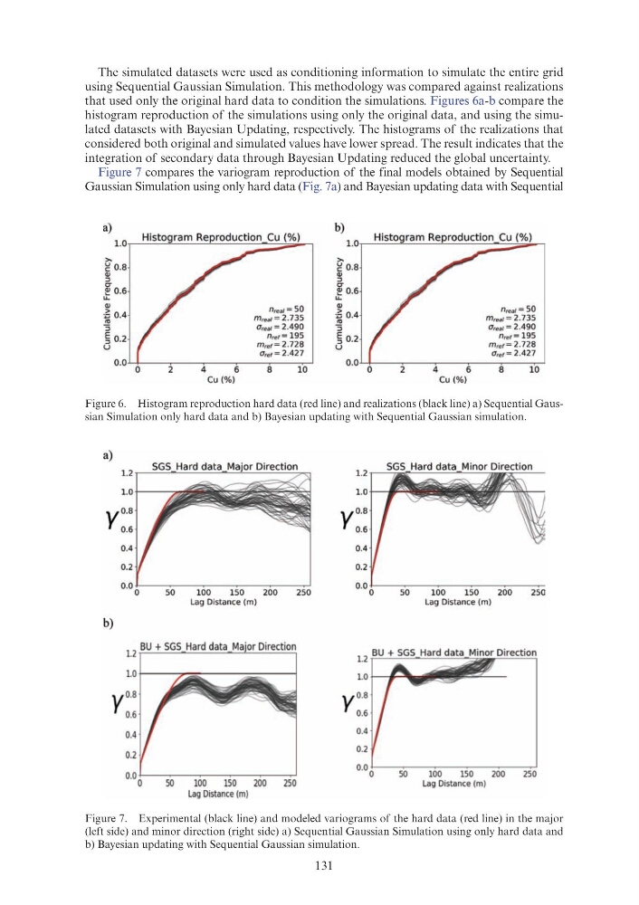
Figure 6. Histogram reproduction hard data (red line) and realizations (black line) a) Sequential Gaussian Simulation only hard data and b) Bayesian updating with Sequential Gaussian simulation.
Figure 7. Experimental (black line) and modeled variograms of the hard data (red line) in the major
(left side) and minor direction (right side) a) Sequential Gaussian Simulation using only hard data and
b) Bayesian updating with Sequential Gaussian simulation.
The simulated datasets were used as conditioning information to simulate the entire grid
using Sequential Gaussian Simulation. This methodology was compared against realizations
that used only the original hard data to condition the simulations. Figures 6a-b compare the
histogram reproduction of the simulations using only the original data, and using the simulated datasets with Bayesian Updating, respectively. The histograms of the realizations that
considered both original and simulated values have lower spread. The result indicates that the
integration of secondary data through Bayesian Updating reduced the global uncertainty.
Figure 7 compares the variogram reproduction of the final models obtained by Sequential
Gaussian Simulation using only hard data (Fig. 7a) and Bayesian updating data with Sequential
a)
,.,
2! 0.8
Qi
::>
cr
~ 0.6
u._
Qi
:5 0.4
.'!?
::>
5 0.2
u
n real = 50
m, •• , = 2. 735
a, •• ,= 2.490
n,.,= 195
m,., = 2.728
a,.,= 2.427
o.o ~----,2 ~--4 ~-~ 6--~ 8 ~---., 1~ 0--'
a)
1.0
YO.B
0.6
0.4
0.2
b)
1.2 BU + SGS
Y0. 8
0.6
0.4
0.2
Cu (%)
Lag Distance (m)
Direction
0.0 +---~-~--~-~----.--'
0
50
100
150
200
250
Lag Distance (m)
b)
,.,
2! 0.8
Qi
::>
cr
~ 0.6
u._
Qi
:5 0.4
.'!?
::>
5 0.2
u
1.2
1.0
y0.8
0.6
0.4
0.2
Y O .B
0.6
0.4
0.2
0.00
2
4
6
Cu (% )
n real =50
m ,.., = 2.735
a,.., = 2.490
n,.,= 195
m,., = 2.728
a,.,= 2.427
8
10
Lag Distance (m)
50
100
150
200
250
Lag Distance (m)