

122
Figure 5 shows two panels on the bench that have been assigned to an Inferred category.
Both panels have been sampled with additional “holes”. In panel C it was necessary to drill
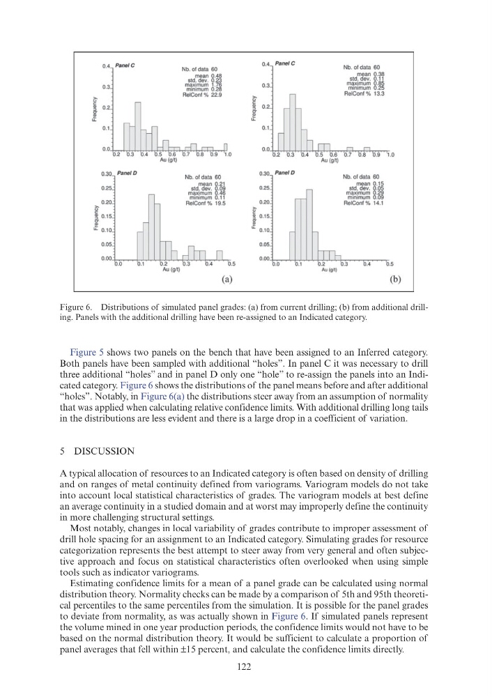
three additional “holes” and in panel D only one “hole” to re-assign the panels into an Indicated category. Figure 6 shows the distributions of the panel means before and after additional
“holes”. Notably, in Figure 6(a) the distributions steer away from an assumption of normality
that was applied when calculating relative confidence limits. With additional drilling long tails
in the distributions are less evident and there is a large drop in a coefficient of variation.
5 DISCUSSION
A typical allocation of resources to an Indicated category is often based on density of drilling
and on ranges of metal continuity defined from variograms. Variogram models do not take
into account local statistical characteristics of grades. The variogram models at best define
an average continuity in a studied domain and at worst may improperly define the continuity
in more challenging structural settings.
Most notably, changes in local variability of grades contribute to improper assessment of
drill hole spacing for an assignment to an Indicated category. Simulating grades for resource
categorization represents the best attempt to steer away from very general and often subjective approach and focus on statistical characteristics often overlooked when using simple
tools such as indicator variograms.
Estimating confidence limits for a mean of a panel grade can be calculated using normal
distribution theory. Normality checks can be made by a comparison of 5th and 95th theoretical percentiles to the same percentiles from the simulation. It is possible for the panel grades
to deviate from normality, as was actually shown in Figure 6. If simulated panels represent
the volume mined in one year production periods, the confidence limits would not have to be
based on the normal distribution theory. It would be sufficient to calculate a proportion of
panel averages that fell within ±15 percent, and calculate the confidence limits directly.
Figure 6. Distributions of simulated panel grades: (a) from current drilling; (b) from additional drilling. Panels with the additional drilling have been re-assigned to an Indicated category.
0.4 Pane/C
0.4 Pane/C
Nb. of data 60
Nb. of data 60
mean 0.48
mean 0.38
std. dev. 0.23
riJ~~~~~ 8:~~
0.3
maximum 1.76
0.3
minimum 0.28
m1mmum 0.25
ReiConf% 22.9
ReiConf% 13.3
g
g
~ 0.2
"
0.2
,_
!
!"
u.
0.1
0.0
0.30 PaneiD
Nb. of data 60
0.30 Pane/D
Nb. of data 60
0.25
mean 0.21
std. dev. 0.09
maximum 0.46
minimum 0.11
0.25
mean 0.15
std. dev. 0.05
maximum 0.29
minimum 0.09
0.20
ReiConf% 19.5
0.20
ReiConf % 14.1
g
g
~ 0.15
~ 0.15
,_
!
.t 0.10
0.10
0.05
0.05
0.00
0.00
lTh
.0
0.1
0.5
b.O
0.1
0.2
0.3
0.4
0.5
Au(g/t)
(a)
(b)
a)
Cu DDH (%)
b)
Cu_Chip (%)
300
11
20
300
250 .. . .. .
250
8.25
15
-200
"E 2oo
E
g' 150
01
5.5
·" 150
10
:c
.c
t::
t
~ 100
~ 100
50
2.75
so
0 .
0
0
100
200
0
0
100
200
0
Easting (m)
Easting (m)
c)
Cu_XRF (%)
15
300
250
11.2
:g 200
Ol
·= 150
~
7 .5
~ 100
50
3.75
0
0
100
200
0
Easting (m)
Figure 5 shows two panels on the bench that have been assigned to an Inferred category.
Both panels have been sampled with additional “holes”. In panel C it was necessary to drill
three additional “holes” and in panel D only one “hole” to re-assign the panels into an Indicated category. Figure 6 shows the distributions of the panel means before and after additional
“holes”. Notably, in Figure 6(a) the distributions steer away from an assumption of normality
that was applied when calculating relative confidence limits. With additional drilling long tails
in the distributions are less evident and there is a large drop in a coefficient of variation.
5 DISCUSSION
A typical allocation of resources to an Indicated category is often based on density of drilling
and on ranges of metal continuity defined from variograms. Variogram models do not take
into account local statistical characteristics of grades. The variogram models at best define
an average continuity in a studied domain and at worst may improperly define the continuity
in more challenging structural settings.
Most notably, changes in local variability of grades contribute to improper assessment of
drill hole spacing for an assignment to an Indicated category. Simulating grades for resource
categorization represents the best attempt to steer away from very general and often subjective approach and focus on statistical characteristics often overlooked when using simple
tools such as indicator variograms.
Estimating confidence limits for a mean of a panel grade can be calculated using normal
distribution theory. Normality checks can be made by a comparison of 5th and 95th theoretical percentiles to the same percentiles from the simulation. It is possible for the panel grades
to deviate from normality, as was actually shown in Figure 6. If simulated panels represent
the volume mined in one year production periods, the confidence limits would not have to be
based on the normal distribution theory. It would be sufficient to calculate a proportion of
panel averages that fell within ±15 percent, and calculate the confidence limits directly.
Figure 6. Distributions of simulated panel grades: (a) from current drilling; (b) from additional drilling. Panels with the additional drilling have been re-assigned to an Indicated category.
0.4 Pane/C
0.4 Pane/C
Nb. of data 60
Nb. of data 60
mean 0.48
mean 0.38
std. dev. 0.23
riJ~~~~~ 8:~~
0.3
maximum 1.76
0.3
minimum 0.28
m1mmum 0.25
ReiConf% 22.9
ReiConf% 13.3
g
g
~ 0.2
"
0.2
,_
!
!"
u.
0.1
0.0
0.30 PaneiD
Nb. of data 60
0.30 Pane/D
Nb. of data 60
0.25
mean 0.21
std. dev. 0.09
maximum 0.46
minimum 0.11
0.25
mean 0.15
std. dev. 0.05
maximum 0.29
minimum 0.09
0.20
ReiConf% 19.5
0.20
ReiConf % 14.1
g
g
~ 0.15
~ 0.15
,_
!
.t 0.10
0.10
0.05
0.05
0.00
0.00
lTh
.0
0.1
0.5
b.O
0.1
0.2
0.3
0.4
0.5
Au(g/t)
(a)
(b)
a)
Cu DDH (%)
b)
Cu_Chip (%)
300
11
20
300
250 .. . .. .
250
8.25
15
-200
"E 2oo
E
g' 150
01
5.5
·" 150
10
:c
.c
t::
t
~ 100
~ 100
50
2.75
so
0 .
0
0
100
200
0
0
100
200
0
Easting (m)
Easting (m)
c)
Cu_XRF (%)
15
300
250
11.2
:g 200
Ol
·= 150
~
7 .5
~ 100
50
3.75
0
0
100
200
0
Easting (m)