

109
patterns in data, ANNs have been proposed as an alternative method for spatial interpolation
(Öztopal, 2006) and (Carvalho et al., 2007). The ANN approach makes no assumptions regarding stationarity, obviates the need to specify a covariance model (Rigol et al., 2001), and can
provide multiple realizations of the estimated field (Rizzo and Dougherty, 1994). This method
can reduce drastically the user influence or even allow a fully automatic workflow. This workflow
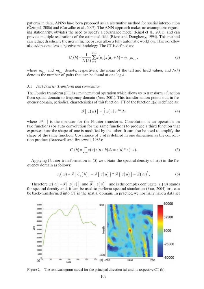
also addresses a less subjective methodology. The CT is defined as:
C
N
z
z
m m
z
C
N
z
z
m
h
h
z
( )
h = ( )
h
( )
u (
)
u h
+
=
( )
h
∑
− h
z
1
1
α
z
) (u
,
(3)
where m z h
−
and m z h
+
denote, respectively, the mean of the tail and head values, and N(h)
denotes the number of pairs that can be found at one lag h.
3.1 Fast Fourier Transform and convolution
The Fourier transform (FT) is a mathematical operation which allows us to transform a function
from spatial domain to frequency domain (Yoo, 2001). This transformation points out, in frequency domain, periodical characteristics of this function. FT of the function z(u) is defined as:
F z
z
e du
d d
i
( )
u
⎡ ⎣ ⎡ ⎡
⎤ ⎦ ⎤ ⎤ =
( )
u
∫
(4)
where F [ ]
⋅ is the operator for the Fourier transform. Convolution is an operation on
two functions (or auto convolution for the same function) to produce a third function that
expresses how the shape of one is modified by the other. It can also be used to amplify the
shape of the same function. Covariance of z(u) is defined in one dimension as the convolution product (Bracewell and Bracewell, 1986):
C
z z
du z
d d
z
C ( )
h =
( )
u (
)
u h
+
( )
u
( )
−∞
∞
∫ −
*
.
z( )
u
−
(5)
Applying Fourier transformation in (5) we obtain the spectral density of z(u) in the frequency domain as follows:
s z
z
z
( )
( )
⎡ ⎣
⎤ ⎦ ⎤ ⎤
( )
u
⎡ ⎣ ⎡ ⎡
⎤ ⎦ ⎤ ⎤
( )
⎡ ⎣
⎤ ⎦
( )
F
F
C z
C z
C ( )
h h
⎡
⎤ ⎤ ⎤
F
,
Z Z
z
*
( )
u
⎡ ⎣ ⎡ ⎡
⎤ ⎦ ⎤ ⎤
( )
ω
F
2
(6)
Therefore Z
z
( )
ω
( )
⎡ ⎣ ⎡ ⎡
⎤ ⎦ ⎤ ⎤
( )
u
⎡ ⎣ ⎡ ⎡
⎤ ⎦ ⎤ ⎤
F
F
z( )
u
⎡ ⎡ ⎡
⎤ ⎤ ⎤ ,
and is the complex conjugate. s z ( )
ω stands
for spectral density and, it can be used to perform spectral simulation (Yao, 2004) orit can
be back-transformed into CT in the spatial domain. In practice, we normally have a data set
Figure 2. The semivariogram model for the principal direction (a) and its respective CT (b).
1>0000
300
60000
60000
50000
60000
32500
.s::;
t:
5000
0
z
1500:1
-25500
10000
"""" G
-50000
(a)
""
ICO
100
lags
patterns in data, ANNs have been proposed as an alternative method for spatial interpolation
(Öztopal, 2006) and (Carvalho et al., 2007). The ANN approach makes no assumptions regarding stationarity, obviates the need to specify a covariance model (Rigol et al., 2001), and can
provide multiple realizations of the estimated field (Rizzo and Dougherty, 1994). This method
can reduce drastically the user influence or even allow a fully automatic workflow. This workflow
also addresses a less subjective methodology. The CT is defined as:
C
N
z
z
m m
z
C
N
z
z
m
h
h
z
( )
h = ( )
h
( )
u (
)
u h
+
=
( )
h
∑
− h
z
1
1
α
z
) (u
,
(3)
where m z h
−
and m z h
+
denote, respectively, the mean of the tail and head values, and N(h)
denotes the number of pairs that can be found at one lag h.
3.1 Fast Fourier Transform and convolution
The Fourier transform (FT) is a mathematical operation which allows us to transform a function
from spatial domain to frequency domain (Yoo, 2001). This transformation points out, in frequency domain, periodical characteristics of this function. FT of the function z(u) is defined as:
F z
z
e du
d d
i
( )
u
⎡ ⎣ ⎡ ⎡
⎤ ⎦ ⎤ ⎤ =
( )
u
∫
(4)
where F [ ]
⋅ is the operator for the Fourier transform. Convolution is an operation on
two functions (or auto convolution for the same function) to produce a third function that
expresses how the shape of one is modified by the other. It can also be used to amplify the
shape of the same function. Covariance of z(u) is defined in one dimension as the convolution product (Bracewell and Bracewell, 1986):
C
z z
du z
d d
z
C ( )
h =
( )
u (
)
u h
+
( )
u
( )
−∞
∞
∫ −
*
.
z( )
u
−
(5)
Applying Fourier transformation in (5) we obtain the spectral density of z(u) in the frequency domain as follows:
s z
z
z
( )
( )
⎡ ⎣
⎤ ⎦ ⎤ ⎤
( )
u
⎡ ⎣ ⎡ ⎡
⎤ ⎦ ⎤ ⎤
( )
⎡ ⎣
⎤ ⎦
( )
F
F
C z
C z
C ( )
h h
⎡
⎤ ⎤ ⎤
F
,
Z Z
z
*
( )
u
⎡ ⎣ ⎡ ⎡
⎤ ⎦ ⎤ ⎤
( )
ω
F
2
(6)
Therefore Z
z
( )
ω
( )
⎡ ⎣ ⎡ ⎡
⎤ ⎦ ⎤ ⎤
( )
u
⎡ ⎣ ⎡ ⎡
⎤ ⎦ ⎤ ⎤
F
F
z( )
u
⎡ ⎡ ⎡
⎤ ⎤ ⎤ ,
and is the complex conjugate. s z ( )
ω stands
for spectral density and, it can be used to perform spectral simulation (Yao, 2004) orit can
be back-transformed into CT in the spatial domain. In practice, we normally have a data set
Figure 2. The semivariogram model for the principal direction (a) and its respective CT (b).
1>0000
300
60000
60000
50000
60000
32500
.s::;
t:
5000
0
z
1500:1
-25500
10000
"""" G
-50000
(a)
""
ICO
100
lags