

80
This can be easily checked by plotting scatterplots and displaying the experimental direct and
cross-variograms.
The simulation process will return as output a suite of L realizations of the normal scores of
the principal components, over a lattice of locations u defined over the simulation domain D:
i
p
l
L
i
;
p
, ,
{
}
Y
u D
i l
Y Y
sim i
,
,u D
( )
u
∀ =
i i
p ∀l
1
1
p p p
(12)
These realizations reproduce a histogram following a standard normal distribution, honor
the data at sample locations Y
i
p
n
i
Y Y
α
( )
u α ∀ =
i
∀ =
α
(
)
, i
∀i
;
p p
, ,
… ,
1
1
p p −
p
1
and reproduce the spatial
continuity imposed by the variogram model (Deutsch and Journel, 1998).
3.5 Back-transformations
The resulting simulated values need to be brought back to their original units by applying
the corresponding normal score, principal component and log-ratio back-transformations.
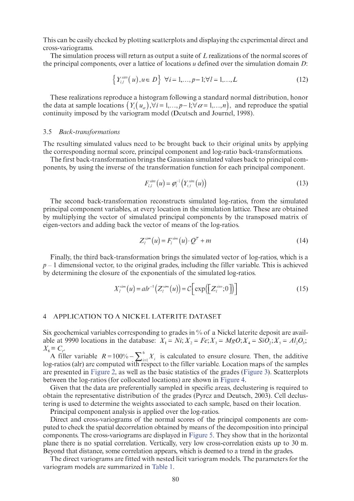
The first back-transformation brings the Gaussian simulated values back to principal components, by using the inverse of the transformation function for each principal component.
F
Y
i l
F F
sim i
i
i
Y Y l
sim i
,
i
,l
i
( )
u =
( )
u
(
)
−
ϕ i
1
(13)
The second back-transformation reconstructs simulated log-ratios, from the simulated
principal component variables, at every location in the simulation lattice. These are obtained
by multiplying the vector of simulated principal components by the transposed matrix of
eigen-vectors and adding back the vector of means of the log-ratios.
Z
F
Q
m
l
Z
sim i
l
F F
si
T
Q
m
i
( )
u =
( )
u
( )
u ⋅Q Q
(14)
Finally, the third back-transformation brings the simulated vector of log-ratios, which is a
p – 1 dimensional vector, to the original grades, including the filler variable. This is achieved
by determining the closure of the exponentials of the simulated log-ratios.
X
alr Z
l l
l
X
sim i
l
Z
sim i i
( )
u =
( )
u
(
)
(
)
Z l
sim i i
⎡ ⎣
⎤ ⎦ ⎤ ⎤
⎡
⎣
⎤
⎦
⎤ ⎤
1
C e p Z l
Z
sim i i
( ⎣ ⎡ ⎡
(15)
4 APPLICATION TO A NICKEL LATERITE DATASET
Six geochemical variables corresponding to grades in % of a Nickel laterite deposit are available at 9990 locations in the database: X Ni X
N N
F X
MgO
M
X
SiO X
Al O
1
2
X N
X
i
N N
3
4
X
M
X
gO
M M
2
5
X
2 3
l O
l O
Ni N Ni N
MgO M MgO M
;
X
Fe
2
X X =
X 2
X
;
;
X
SiO
4
X
2
O O
X X
;
X 6 = C r .
A filler variable R
X i
X
i =
∑
00
100
1
6
%
is calculated to ensure closure. Then, the additive
log-ratios (alr) are computed with respect to the filler variable. Location maps of the samples
are presented in Figure 2, as well as the basic statistics of the grades (Figure 3). Scatterplots
between the log-ratios (for collocated locations) are shown in Figure 4.
Given that the data are preferentially sampled in specific areas, declustering is required to
obtain the representative distribution of the grades (Pyrcz and Deutsch, 2003). Cell declustering is used to determine the weights associated to each sample, based on their location.
Principal component analysis is applied over the log-ratios.
Direct and cross-variograms of the normal scores of the principal components are computed to check the spatial decorrelation obtained by means of the decomposition into principal
components. The cross-variograms are displayed in Figure 5. They show that in the horizontal
plane there is no spatial correlation. Vertically, very low cross-correlation exists up to 30 m.
Beyond that distance, some correlation appears, which is deemed to a trend in the grades.
The direct variograms are fitted with nested licit variogram models. The parameters for the
variogram models are summarized in Table 1.
This can be easily checked by plotting scatterplots and displaying the experimental direct and
cross-variograms.
The simulation process will return as output a suite of L realizations of the normal scores of
the principal components, over a lattice of locations u defined over the simulation domain D:
i
p
l
L
i
;
p
, ,
{
}
Y
u D
i l
Y Y
sim i
,
,u D
( )
u
∀ =
i i
p ∀l
1
1
p p p
(12)
These realizations reproduce a histogram following a standard normal distribution, honor
the data at sample locations Y
i
p
n
i
Y Y
α
( )
u α ∀ =
i
∀ =
α
(
)
, i
∀i
;
p p
, ,
… ,
1
1
p p −
p
1
and reproduce the spatial
continuity imposed by the variogram model (Deutsch and Journel, 1998).
3.5 Back-transformations
The resulting simulated values need to be brought back to their original units by applying
the corresponding normal score, principal component and log-ratio back-transformations.
The first back-transformation brings the Gaussian simulated values back to principal components, by using the inverse of the transformation function for each principal component.
F
Y
i l
F F
sim i
i
i
Y Y l
sim i
,
i
,l
i
( )
u =
( )
u
(
)
−
ϕ i
1
(13)
The second back-transformation reconstructs simulated log-ratios, from the simulated
principal component variables, at every location in the simulation lattice. These are obtained
by multiplying the vector of simulated principal components by the transposed matrix of
eigen-vectors and adding back the vector of means of the log-ratios.
Z
F
Q
m
l
Z
sim i
l
F F
si
T
Q
m
i
( )
u =
( )
u
( )
u ⋅Q Q
(14)
Finally, the third back-transformation brings the simulated vector of log-ratios, which is a
p – 1 dimensional vector, to the original grades, including the filler variable. This is achieved
by determining the closure of the exponentials of the simulated log-ratios.
X
alr Z
l l
l
X
sim i
l
Z
sim i i
( )
u =
( )
u
(
)
(
)
Z l
sim i i
⎡ ⎣
⎤ ⎦ ⎤ ⎤
⎡
⎣
⎤
⎦
⎤ ⎤
1
C e p Z l
Z
sim i i
( ⎣ ⎡ ⎡
(15)
4 APPLICATION TO A NICKEL LATERITE DATASET
Six geochemical variables corresponding to grades in % of a Nickel laterite deposit are available at 9990 locations in the database: X Ni X
N N
F X
MgO
M
X
SiO X
Al O
1
2
X N
X
i
N N
3
4
X
M
X
gO
M M
2
5
X
2 3
l O
l O
Ni N Ni N
MgO M MgO M
;
X
Fe
2
X X =
X 2
X
;
;
X
SiO
4
X
2
O O
X X
;
X 6 = C r .
A filler variable R
X i
X
i =
∑
00
100
1
6
%
is calculated to ensure closure. Then, the additive
log-ratios (alr) are computed with respect to the filler variable. Location maps of the samples
are presented in Figure 2, as well as the basic statistics of the grades (Figure 3). Scatterplots
between the log-ratios (for collocated locations) are shown in Figure 4.
Given that the data are preferentially sampled in specific areas, declustering is required to
obtain the representative distribution of the grades (Pyrcz and Deutsch, 2003). Cell declustering is used to determine the weights associated to each sample, based on their location.
Principal component analysis is applied over the log-ratios.
Direct and cross-variograms of the normal scores of the principal components are computed to check the spatial decorrelation obtained by means of the decomposition into principal
components. The cross-variograms are displayed in Figure 5. They show that in the horizontal
plane there is no spatial correlation. Vertically, very low cross-correlation exists up to 30 m.
Beyond that distance, some correlation appears, which is deemed to a trend in the grades.
The direct variograms are fitted with nested licit variogram models. The parameters for the
variogram models are summarized in Table 1.