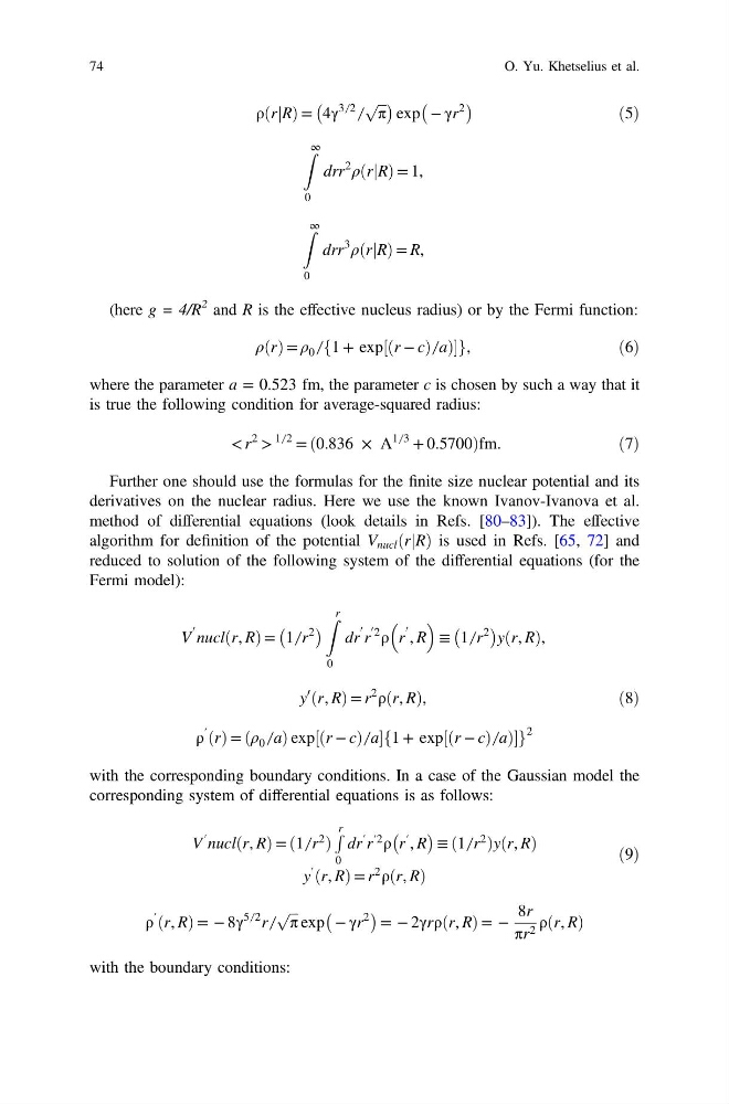
ρ rjR
ð Þ= 4γ
3 ̸ 2
̸
ffiffi ffi
π
p
À
Á
exp − γr
2
À
Á
ð5Þ
Z ∞
0
drr
2
ρ rjR
ð Þ= 1,
Z ∞
0
drr
3
ρ rjR
ð Þ= R,
(here g = 4/R
2 and R is the effective nucleus radius) or by the Fermi function:
ρðrÞ = ρ 0 ̸ f1 + exp½ðr − cÞ ̸ aފg,
ð6Þ
where the parameter a = 0.523 fm, the parameter c is chosen by such a way that it
is true the following condition for average-squared radius:
< r
2 >
1 ̸ 2 = ð0.836 × A
1 ̸ 3 + 0.5700Þfm.
ð7Þ
Further one should use the formulas for the finite size nuclear potential and its
derivatives on the nuclear radius. Here we use the known Ivanov-Ivanova et al.
method of differential equations (look details in Refs. [80–83]). The effective
algorithm for definition of the potential V nucl rjR
ð Þ is used in Refs. [65, 72] and
reduced to solution of the following system of the differential equations (for the
Fermi model):
V
0 nucl r, R
ð Þ= 1 ̸ r
2
À
Á
Z r
0
dr
0 r
0 2
ρ r
0 , R
≡ 1 ̸ r
2
À
Á
y r, R
ð Þ,
y
0 r, R
ð Þ= r
2
ρ r, R
ð Þ,
ð8Þ
ρ
′
ðrÞ = ðρ 0 ̸ aÞ exp½ðr − cÞ ̸ aŠf1 + exp½ðr − cÞ ̸ aފg
2
with the corresponding boundary conditions. In a case of the Gaussian model the
corresponding system of differential equations is as follows:
V
′ nucl r, R
ð Þ= 1 ̸ r
2
ð
Þ
R r
0
dr
′ r
′2
ρ r
′ , R
À
Á ≡ 1 ̸ r
2
ð
Þy r, R
ð Þ
y
′ r, R
ð Þ= r
2
ρ r, R
ð Þ
ð9Þ
ρ
′ r, R
ð Þ= − 8γ
5 ̸ 2 r ̸
ffiffi ffi
π
p
exp − γr
2
À
Á
= − 2γrρ r, R
ð Þ= −
8r
πr 2 ρ r, R
ð Þ
with the boundary conditions:
74
O. Yu. Khetselius et al.