

Matrix Elements for Explicitly-Correlated Atomic Wave Functions
35
̂
í µí°« 1 ⋅ ̂
í µí°« 12 =
r
2
1
+ r
2
12
− r
2
2
2r 1 r 12
,
(15)
0 = ∇ 1 g d (1) ⋅ ∇ 1 Y
m
l
(1) .
(16)
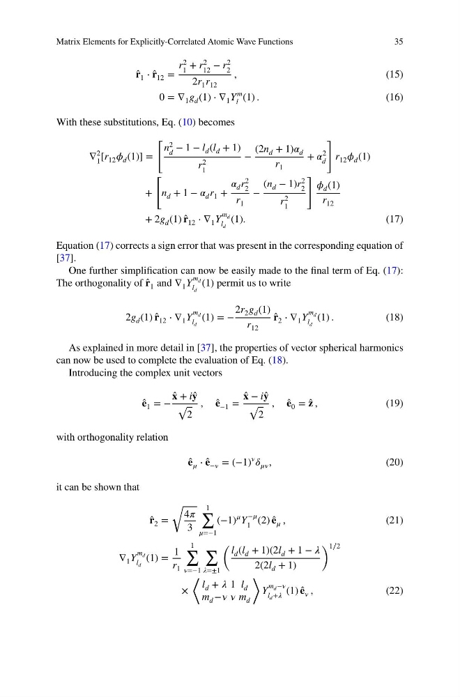
With these substitutions, Eq. (10) becomes
∇
2
1 [r 12 í µí¼ d (1)] =
[
n
2
d
− 1 − l d (l d + 1)
r
2
1
−
(2n d + 1)í µí»¼ d
r 1
+ í µí»¼
2
d
]
r 12 í µí¼ d (1)
+
[
n d + 1 − í µí»¼ d r 1 +
í µí»¼ d r
2
2
r 1
−
(n d − 1)r
2
2
r
2
1
]
í µí¼ d (1)
r 12
+ 2g d (1) ̂
í µí°« 12 ⋅ ∇ 1 Y
m d
l d
(1).
(17)
Equation (17) corrects a sign error that was present in the corresponding equation of
[37].
One further simplification can now be easily made to the final term of Eq. (17):
The orthogonality of ̂
í µí°« 1 and ∇ 1 Y
m d
l d
(1) permit us to write
2g d (1) ̂
í µí°« 12 ⋅ ∇ 1 Y
m d
l d
(1) = −
2r 2 g d (1)
r 12
̂
í µí°« 2 ⋅ ∇ 1 Y
m d
l d
(1) .
(18)
As explained in more detail in [37], the properties of vector spherical harmonics
can now be used to complete the evaluation of Eq. (18).
Introducing the complex unit vectors
̂
í µí° 1 = −
̂
í µí°± + i ̂
í µí°²
√
2
, ̂
í µí° −1 =
̂
í µí°± − i ̂
í µí°²
√
2
, ̂
í µí° 0 = ̂
í µí°³ ,
(19)
with orthogonality relation
̂
í µí° í µí¼ ⋅ ̂
í µí° −í µí¼ = (−1)
í µí¼
í µí»¿ í µí¼í µí¼ ,
(20)
it can be shown that
̂
í µí°« 2 =
√
4í µí¼
3
1
∑
í µí¼=−1
(−1)
í µí¼ Y
−í µí¼
1
(2) ̂
í µí° í µí¼ ,
(21)
∇ 1 Y
m d
l d
(1) =
1
r 1
1
∑
í µí¼=−1
∑
í µí¼=±1
( l d (l d + 1)(2l d + 1 − í µí¼
2(2l d + 1)
) 1∕2
×
⟨
l d + í µí¼ 1 l d
m d −í µí¼ í µí¼ m d
⟩
Y
m d −í µí¼
l d +í µí¼
(1) ̂
í µí° í µí¼ ,
(22)
35
̂
í µí°« 1 ⋅ ̂
í µí°« 12 =
r
2
1
+ r
2
12
− r
2
2
2r 1 r 12
,
(15)
0 = ∇ 1 g d (1) ⋅ ∇ 1 Y
m
l
(1) .
(16)
With these substitutions, Eq. (10) becomes
∇
2
1 [r 12 í µí¼ d (1)] =
[
n
2
d
− 1 − l d (l d + 1)
r
2
1
−
(2n d + 1)í µí»¼ d
r 1
+ í µí»¼
2
d
]
r 12 í µí¼ d (1)
+
[
n d + 1 − í µí»¼ d r 1 +
í µí»¼ d r
2
2
r 1
−
(n d − 1)r
2
2
r
2
1
]
í µí¼ d (1)
r 12
+ 2g d (1) ̂
í µí°« 12 ⋅ ∇ 1 Y
m d
l d
(1).
(17)
Equation (17) corrects a sign error that was present in the corresponding equation of
[37].
One further simplification can now be easily made to the final term of Eq. (17):
The orthogonality of ̂
í µí°« 1 and ∇ 1 Y
m d
l d
(1) permit us to write
2g d (1) ̂
í µí°« 12 ⋅ ∇ 1 Y
m d
l d
(1) = −
2r 2 g d (1)
r 12
̂
í µí°« 2 ⋅ ∇ 1 Y
m d
l d
(1) .
(18)
As explained in more detail in [37], the properties of vector spherical harmonics
can now be used to complete the evaluation of Eq. (18).
Introducing the complex unit vectors
̂
í µí° 1 = −
̂
í µí°± + i ̂
í µí°²
√
2
, ̂
í µí° −1 =
̂
í µí°± − i ̂
í µí°²
√
2
, ̂
í µí° 0 = ̂
í µí°³ ,
(19)
with orthogonality relation
̂
í µí° í µí¼ ⋅ ̂
í µí° −í µí¼ = (−1)
í µí¼
í µí»¿ í µí¼í µí¼ ,
(20)
it can be shown that
̂
í µí°« 2 =
√
4í µí¼
3
1
∑
í µí¼=−1
(−1)
í µí¼ Y
−í µí¼
1
(2) ̂
í µí° í µí¼ ,
(21)
∇ 1 Y
m d
l d
(1) =
1
r 1
1
∑
í µí¼=−1
∑
í µí¼=±1
( l d (l d + 1)(2l d + 1 − í µí¼
2(2l d + 1)
) 1∕2
×
⟨
l d + í µí¼ 1 l d
m d −í µí¼ í µí¼ m d
⟩
Y
m d −í µí¼
l d +í µí¼
(1) ̂
í µí° í µí¼ ,
(22)