

346
P. Xiang and Y. A. Wang
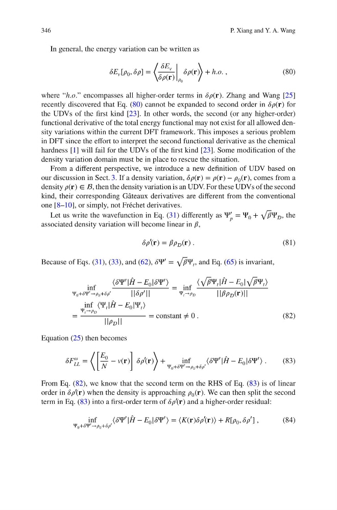
In general, the energy variation can be written as
í µí»¿E v [í µí¼ 0 , í µí»¿í µí¼] =
⟨ í µí»¿E v
í µí»¿í µí¼(í µí°«)
|
|
|
|í µí¼ 0
í µí»¿í µí¼(í µí°«)
⟩
+ h.o. ,
(80)
where “h.o.” encompasses all higher-order terms in í µí»¿í µí¼(í µí°«). Zhang and Wang [25]
recently discovered that Eq. (80) cannot be expanded to second order in í µí»¿í µí¼(í µí°«) for
the UDVs of the first kind [23]. In other words, the second (or any higher-order)
functional derivative of the total energy functional may not exist for all allowed density variations within the current DFT framework. This imposes a serious problem
in DFT since the effort to interpret the second functional derivative as the chemical
hardness [1] will fail for the UDVs of the first kind [23]. Some modification of the
density variation domain must be in place to rescue the situation.
From a different perspective, we introduce a new definition of UDV based on
our discussion in Sect. 3. If a density variation, í µí»¿í µí¼(í µí°«) = í µí¼(í µí°«) − í µí¼ 0 (í µí°«), comes from a
density í µí¼(í µí°«) ∈ , then the density variation is an UDV. For these UDVs of the second
kind, their corresponding Gâteaux derivatives are different from the conventional
one [8–10], or simply, not Fréchet derivatives.
Let us write the wavefunction in Eq. (31) differently as Ψ ′
p = Ψ 0 +
√
í µí»½Ψ , the
associated density variation will become linear in í µí»½,
í µí»¿í µí¼
′
(í µí°«) = í µí»½í µí¼ (í µí°«) .
(81)
Because of Eqs. (31), (33), and (62), í µí»¿Ψ ′ =
√ í µí»½Ψ t , and Eq. (65) is invariant,
inf
Ψ 0 +í µí»¿Ψ ′ →í µí¼ 0 +í µí»¿í µí¼ ′
⟨í µí»¿Ψ ′ | ̂
H − E 0 |í µí»¿Ψ ′ ⟩
||í µí»¿í µí¼ ′ ||
= inf
Ψ t →í µí¼
⟨
√
í µí»½Ψ t | ̂
H − E 0 |
√
í µí»½Ψ t ⟩
||í µí»½í µí¼ (í µí°«)||
=
inf
Ψ t →í µí¼
⟨Ψ t | ̂
H − E 0 |Ψ t ⟩
||í µí¼ ||
= constant ≠ 0 .
(82)
Equation (25) then becomes
í µí»¿F
í µí¼
LL =
⟨[ E 0
N
− v(í µí°«)
]
í µí»¿í µí¼
′
(í µí°«)
⟩
+
inf
Ψ 0 +í µí»¿Ψ ′ →í µí¼ 0 +í µí»¿í µí¼ ′
⟨í µí»¿Ψ
′
| ̂
H − E 0 |í µí»¿Ψ
′
⟩ .
(83)
From Eq. (82), we know that the second term on the RHS of Eq. (83) is of linear
order in í µí»¿í µí¼ ′ (í µí°«) when the density is approaching í µí¼ 0 (í µí°«). We can then split the second
term in Eq. (83) into a first-order term of í µí»¿í µí¼
′
(í µí°«) and a higher-order residual:
inf
Ψ 0 +í µí»¿Ψ ′ →í µí¼ 0 +í µí»¿í µí¼ ′
⟨í µí»¿Ψ
′
| ̂
H − E 0 |í µí»¿Ψ
′
⟩ = ⟨K(í µí°«)í µí»¿í µí¼
′
(í µí°«)⟩ + R[í µí¼ 0 , í µí»¿í µí¼
′
] ,
(84)
P. Xiang and Y. A. Wang
In general, the energy variation can be written as
í µí»¿E v [í µí¼ 0 , í µí»¿í µí¼] =
⟨ í µí»¿E v
í µí»¿í µí¼(í µí°«)
|
|
|
|í µí¼ 0
í µí»¿í µí¼(í µí°«)
⟩
+ h.o. ,
(80)
where “h.o.” encompasses all higher-order terms in í µí»¿í µí¼(í µí°«). Zhang and Wang [25]
recently discovered that Eq. (80) cannot be expanded to second order in í µí»¿í µí¼(í µí°«) for
the UDVs of the first kind [23]. In other words, the second (or any higher-order)
functional derivative of the total energy functional may not exist for all allowed density variations within the current DFT framework. This imposes a serious problem
in DFT since the effort to interpret the second functional derivative as the chemical
hardness [1] will fail for the UDVs of the first kind [23]. Some modification of the
density variation domain must be in place to rescue the situation.
From a different perspective, we introduce a new definition of UDV based on
our discussion in Sect. 3. If a density variation, í µí»¿í µí¼(í µí°«) = í µí¼(í µí°«) − í µí¼ 0 (í µí°«), comes from a
density í µí¼(í µí°«) ∈ , then the density variation is an UDV. For these UDVs of the second
kind, their corresponding Gâteaux derivatives are different from the conventional
one [8–10], or simply, not Fréchet derivatives.
Let us write the wavefunction in Eq. (31) differently as Ψ ′
p = Ψ 0 +
√
í µí»½Ψ , the
associated density variation will become linear in í µí»½,
í µí»¿í µí¼
′
(í µí°«) = í µí»½í µí¼ (í µí°«) .
(81)
Because of Eqs. (31), (33), and (62), í µí»¿Ψ ′ =
√ í µí»½Ψ t , and Eq. (65) is invariant,
inf
Ψ 0 +í µí»¿Ψ ′ →í µí¼ 0 +í µí»¿í µí¼ ′
⟨í µí»¿Ψ ′ | ̂
H − E 0 |í µí»¿Ψ ′ ⟩
||í µí»¿í µí¼ ′ ||
= inf
Ψ t →í µí¼
⟨
√
í µí»½Ψ t | ̂
H − E 0 |
√
í µí»½Ψ t ⟩
||í µí»½í µí¼ (í µí°«)||
=
inf
Ψ t →í µí¼
⟨Ψ t | ̂
H − E 0 |Ψ t ⟩
||í µí¼ ||
= constant ≠ 0 .
(82)
Equation (25) then becomes
í µí»¿F
í µí¼
LL =
⟨[ E 0
N
− v(í µí°«)
]
í µí»¿í µí¼
′
(í µí°«)
⟩
+
inf
Ψ 0 +í µí»¿Ψ ′ →í µí¼ 0 +í µí»¿í µí¼ ′
⟨í µí»¿Ψ
′
| ̂
H − E 0 |í µí»¿Ψ
′
⟩ .
(83)
From Eq. (82), we know that the second term on the RHS of Eq. (83) is of linear
order in í µí»¿í µí¼ ′ (í µí°«) when the density is approaching í µí¼ 0 (í µí°«). We can then split the second
term in Eq. (83) into a first-order term of í µí»¿í µí¼
′
(í µí°«) and a higher-order residual:
inf
Ψ 0 +í µí»¿Ψ ′ →í µí¼ 0 +í µí»¿í µí¼ ′
⟨í µí»¿Ψ
′
| ̂
H − E 0 |í µí»¿Ψ
′
⟩ = ⟨K(í µí°«)í µí»¿í µí¼
′
(í µí°«)⟩ + R[í µí¼ 0 , í µí»¿í µí¼
′
] ,
(84)