

338
P. Xiang and Y. A. Wang
where Ψ t is normalized to 1 and í µí¼ is a real scaling parameter (potentially different
from í µí»½). We can expand Ψ t in terms of the complete set of normalized eigenfunctions
{Ψ i } of ̂
H,
Ψ t =
∞
∑
i=0
c i Ψ i ,
(34)
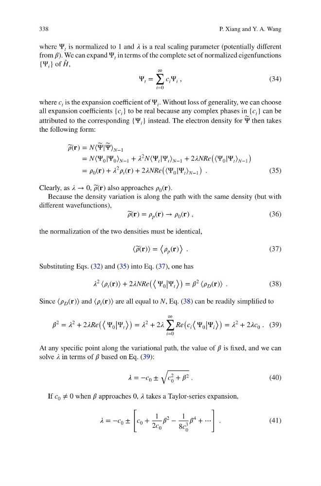
where c i is the expansion coefficient of Ψ i . Without loss of generality, we can choose
all expansion coefficients {c i } to be real because any complex phases in {c i } can be
attributed to the corresponding {Ψ i } instead. The electron density for ̃
Ψ then takes
the following form:
̃
í µí¼(í µí°«) = N⟨ ̃
Ψ| ̃
Ψ⟩ N−1
= N⟨Ψ 0 |Ψ 0 ⟩ N−1 + í µí¼
2 N⟨Ψ t |Ψ t ⟩ N−1 + 2í µí¼NRe
( ⟨Ψ 0 |Ψ t ⟩ N−1
)
= í µí¼ 0 (í µí°«) + í µí¼
2
í µí¼ t (í µí°«) + 2í µí¼NRe
( ⟨Ψ 0 |Ψ t ⟩ N−1
) .
(35)
Clearly, as í µí¼ → 0, ̃
í µí¼(í µí°«) also approaches í µí¼ 0 (í µí°«).
Because the density variation is along the path with the same density (but with
different wavefunctions),
̃
í µí¼(í µí°«) = í µí¼ p (í µí°«) → í µí¼ 0 (í µí°«) ,
(36)
the normalization of the two densities must be identical,
⟨̃ í µí¼(í µí°«)⟩ =
⟨
í µí¼ p (í µí°«)
⟩ .
(37)
Substituting Eqs. (32) and (35) into Eq. (37), one has
í µí¼
2
⟨í µí¼ t (í µí°«)⟩ + 2í µí¼NRe
(⟨ Ψ 0 |
| Ψ t
⟩) = í µí»½
2
⟨í µí¼ (í µí°«)⟩ .
(38)
Since ⟨í µí¼ (í µí°«)⟩ and ⟨í µí¼ t (í µí°«)⟩ are all equal to N, Eq. (38) can be readily simplified to
í µí»½
2
= í µí¼
2
+ 2í µí¼Re
(⟨ Ψ 0
|
| Ψ t
⟩) = í µí¼
2
+ 2í µí¼
∞
∑
i=0
Re
(
c i
⟨ Ψ 0
|
| Ψ i
⟩) = í µí¼
2
+ 2í µí¼c 0 . (39)
At any specific point along the variational path, the value of í µí»½ is fixed, and we can
solve í µí¼ in terms of í µí»½ based on Eq. (39):
í µí¼ = −c 0 ±
√
c
2
0
+ í µí»½ 2 .
(40)
If c 0 ≠ 0 when í µí»½ approaches 0, í µí¼ takes a Taylor-series expansion,
í µí¼ = −c 0 ±
[
c 0 +
1
2c 0
í µí»½
2
−
1
8c
3
0
í µí»½
4
+ ⋯
]
.
(41)
P. Xiang and Y. A. Wang
where Ψ t is normalized to 1 and í µí¼ is a real scaling parameter (potentially different
from í µí»½). We can expand Ψ t in terms of the complete set of normalized eigenfunctions
{Ψ i } of ̂
H,
Ψ t =
∞
∑
i=0
c i Ψ i ,
(34)
where c i is the expansion coefficient of Ψ i . Without loss of generality, we can choose
all expansion coefficients {c i } to be real because any complex phases in {c i } can be
attributed to the corresponding {Ψ i } instead. The electron density for ̃
Ψ then takes
the following form:
̃
í µí¼(í µí°«) = N⟨ ̃
Ψ| ̃
Ψ⟩ N−1
= N⟨Ψ 0 |Ψ 0 ⟩ N−1 + í µí¼
2 N⟨Ψ t |Ψ t ⟩ N−1 + 2í µí¼NRe
( ⟨Ψ 0 |Ψ t ⟩ N−1
)
= í µí¼ 0 (í µí°«) + í µí¼
2
í µí¼ t (í µí°«) + 2í µí¼NRe
( ⟨Ψ 0 |Ψ t ⟩ N−1
) .
(35)
Clearly, as í µí¼ → 0, ̃
í µí¼(í µí°«) also approaches í µí¼ 0 (í µí°«).
Because the density variation is along the path with the same density (but with
different wavefunctions),
̃
í µí¼(í µí°«) = í µí¼ p (í µí°«) → í µí¼ 0 (í µí°«) ,
(36)
the normalization of the two densities must be identical,
⟨̃ í µí¼(í µí°«)⟩ =
⟨
í µí¼ p (í µí°«)
⟩ .
(37)
Substituting Eqs. (32) and (35) into Eq. (37), one has
í µí¼
2
⟨í µí¼ t (í µí°«)⟩ + 2í µí¼NRe
(⟨ Ψ 0 |
| Ψ t
⟩) = í µí»½
2
⟨í µí¼ (í µí°«)⟩ .
(38)
Since ⟨í µí¼ (í µí°«)⟩ and ⟨í µí¼ t (í µí°«)⟩ are all equal to N, Eq. (38) can be readily simplified to
í µí»½
2
= í µí¼
2
+ 2í µí¼Re
(⟨ Ψ 0
|
| Ψ t
⟩) = í µí¼
2
+ 2í µí¼
∞
∑
i=0
Re
(
c i
⟨ Ψ 0
|
| Ψ i
⟩) = í µí¼
2
+ 2í µí¼c 0 . (39)
At any specific point along the variational path, the value of í µí»½ is fixed, and we can
solve í µí¼ in terms of í µí»½ based on Eq. (39):
í µí¼ = −c 0 ±
√
c
2
0
+ í µí»½ 2 .
(40)
If c 0 ≠ 0 when í µí»½ approaches 0, í µí¼ takes a Taylor-series expansion,
í µí¼ = −c 0 ±
[
c 0 +
1
2c 0
í µí»½
2
−
1
8c
3
0
í µí»½
4
+ ⋯
]
.
(41)