

336
P. Xiang and Y. A. Wang
í µí»¿F
í µí¼
LL
= F
í µí¼
LL
[í µí¼ 0 + í µí»¿í µí¼] − F
í µí¼
LL
[í µí¼ 0 ]
=
⟨[ E 0
N
− v(í µí°«)
]
í µí»¿í µí¼(í µí°«)
⟩
+
inf
Ψ 0 +í µí»¿Ψ→í µí¼ 0 +í µí»¿í µí¼
⟨í µí»¿Ψ| ̂
H − E 0 |í µí»¿Ψ⟩ .
(25)
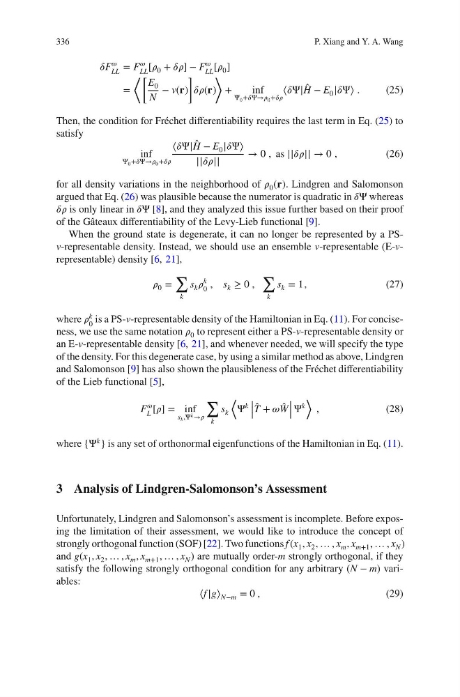
Then, the condition for Fréchet differentiability requires the last term in Eq. (25) to
satisfy
inf
Ψ 0 +í µí»¿Ψ→í µí¼ 0 +í µí»¿í µí¼
⟨í µí»¿Ψ| ̂
H − E 0 |í µí»¿Ψ⟩
||í µí»¿í µí¼||
→ 0 , as ||í µí»¿í µí¼|| → 0 ,
(26)
for all density variations in the neighborhood of í µí¼ 0 (í µí°«). Lindgren and Salomonson
argued that Eq. (26) was plausible because the numerator is quadratic in í µí»¿Ψ whereas
í µí»¿í µí¼ is only linear in í µí»¿Ψ [8], and they analyzed this issue further based on their proof
of the Gâteaux differentiability of the Levy-Lieb functional [9].
When the ground state is degenerate, it can no longer be represented by a PSv-representable density. Instead, we should use an ensemble v-representable (E-vrepresentable) density [6, 21],
í µí¼ 0 =
∑
k
s k í µí¼
k
0
, s k ≥ 0 ,
∑
k
s k = 1,
(27)
where í µí¼
k
0
is a PS-v-representable density of the Hamiltonian in Eq. (11). For conciseness, we use the same notation í µí¼ 0 to represent either a PS-v-representable density or
an E-v-representable density [6, 21], and whenever needed, we will specify the type
of the density. For this degenerate case, by using a similar method as above, Lindgren
and Salomonson [9] has also shown the plausibleness of the Fréchet differentiability
of the Lieb functional [5],
F
í µí¼
L
[í µí¼] = inf
s k ,Ψ k →í µí¼
∑
k
s k
⟨
Ψ
k |
|
|
̂
T + í µí¼ ̂
W
|
|
|
Ψ
k
⟩
,
(28)
where {Ψ k } is any set of orthonormal eigenfunctions of the Hamiltonian in Eq. (11).
3 Analysis of Lindgren-Salomonson’s Assessment
Unfortunately, Lindgren and Salomonson’s assessment is incomplete. Before exposing the limitation of their assessment, we would like to introduce the concept of
strongly orthogonal function (SOF) [22]. Two functions f (x 1 , x 2 , … , x m , x m+1 , … , x N )
and g(x 1 , x 2 , … , x m , x m+1 , … , x N ) are mutually order-m strongly orthogonal, if they
satisfy the following strongly orthogonal condition for any arbitrary (N − m) variables:
⟨f |g⟩ N−m = 0 ,
(29)
P. Xiang and Y. A. Wang
í µí»¿F
í µí¼
LL
= F
í µí¼
LL
[í µí¼ 0 + í µí»¿í µí¼] − F
í µí¼
LL
[í µí¼ 0 ]
=
⟨[ E 0
N
− v(í µí°«)
]
í µí»¿í µí¼(í µí°«)
⟩
+
inf
Ψ 0 +í µí»¿Ψ→í µí¼ 0 +í µí»¿í µí¼
⟨í µí»¿Ψ| ̂
H − E 0 |í µí»¿Ψ⟩ .
(25)
Then, the condition for Fréchet differentiability requires the last term in Eq. (25) to
satisfy
inf
Ψ 0 +í µí»¿Ψ→í µí¼ 0 +í µí»¿í µí¼
⟨í µí»¿Ψ| ̂
H − E 0 |í µí»¿Ψ⟩
||í µí»¿í µí¼||
→ 0 , as ||í µí»¿í µí¼|| → 0 ,
(26)
for all density variations in the neighborhood of í µí¼ 0 (í µí°«). Lindgren and Salomonson
argued that Eq. (26) was plausible because the numerator is quadratic in í µí»¿Ψ whereas
í µí»¿í µí¼ is only linear in í µí»¿Ψ [8], and they analyzed this issue further based on their proof
of the Gâteaux differentiability of the Levy-Lieb functional [9].
When the ground state is degenerate, it can no longer be represented by a PSv-representable density. Instead, we should use an ensemble v-representable (E-vrepresentable) density [6, 21],
í µí¼ 0 =
∑
k
s k í µí¼
k
0
, s k ≥ 0 ,
∑
k
s k = 1,
(27)
where í µí¼
k
0
is a PS-v-representable density of the Hamiltonian in Eq. (11). For conciseness, we use the same notation í µí¼ 0 to represent either a PS-v-representable density or
an E-v-representable density [6, 21], and whenever needed, we will specify the type
of the density. For this degenerate case, by using a similar method as above, Lindgren
and Salomonson [9] has also shown the plausibleness of the Fréchet differentiability
of the Lieb functional [5],
F
í µí¼
L
[í µí¼] = inf
s k ,Ψ k →í µí¼
∑
k
s k
⟨
Ψ
k |
|
|
̂
T + í µí¼ ̂
W
|
|
|
Ψ
k
⟩
,
(28)
where {Ψ k } is any set of orthonormal eigenfunctions of the Hamiltonian in Eq. (11).
3 Analysis of Lindgren-Salomonson’s Assessment
Unfortunately, Lindgren and Salomonson’s assessment is incomplete. Before exposing the limitation of their assessment, we would like to introduce the concept of
strongly orthogonal function (SOF) [22]. Two functions f (x 1 , x 2 , … , x m , x m+1 , … , x N )
and g(x 1 , x 2 , … , x m , x m+1 , … , x N ) are mutually order-m strongly orthogonal, if they
satisfy the following strongly orthogonal condition for any arbitrary (N − m) variables:
⟨f |g⟩ N−m = 0 ,
(29)