

Theor Chem Acc (2015) 134:138
1 3
[ 54 , 55 ] or environmental effects [ 55 ] among others. Therefore, the Hamiltonian in the adiabatic approximation [ 56 ]
for each of the two branches,
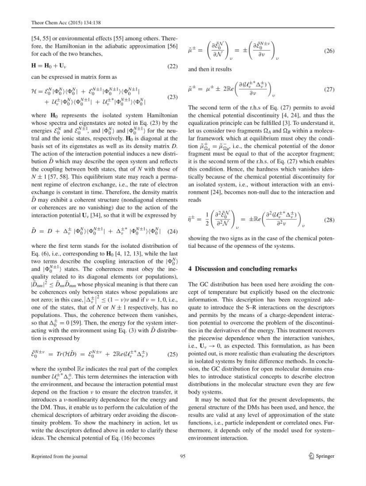
can be expressed in matrix form as
where H 0 represents the isolated system Hamiltonian
whose spectra and eigenstates are noted in Eq. ( 23 ) by the
energies E
N
0 and E
N±1
0
, and |
N
0 and |
N±1
0
for the neutral and the ionic states, respectively. H 0 is diagonal at the
basis set of its eigenstates as well as its density matrix D .
The action of the interaction potential induces a new distribution ˜
D which may describe the open system and refl ects
the coupling between both states, that of N with those of
N ± 1 [ 57 , 58 ]. This equilibrium state may reach a permanent regime of electron exchange, i.e., the rate of electron
exchange is constant in time. Therefore, the density matrix
˜
D may exhibit a coherent structure (nondiagonal elements
or coherences are no vanishing) due to the action of the
interaction potential U ν [ 34 ], so that it will be expressed by
where the fi rst term stands for the isolated distribution of
Eq. ( 6 ), i.e., corresponding to H 0 [ 4 , 12 , 13 ], while the last
two terms describe the coupling interaction of the |
N
0
and |
N±1
0
states. The coherences must obey the inequality related to its diagonal elements (or populations),
| ˜
D nm | 2 ≤ ˜
D nn ˜
D mm whose physical meaning is that there can
be coherences only between states whose populations are
not zero; in this case,
±
ν
2 ≤ (1 − ν)ν and if ν = 1, 0 , i.e.,
one of the states, that of N or N ± 1 respectively, has no
populations. Thus, the coherence between them vanishes,
so that
±
0 = 0 [ 59 ]. Then, the energy for the system interacting with the environment using Eq. ( 3 ) with ˜
D distribution is expressed by
where the symbol Re indicates the real part of the complex
number U ±
ν
∗ ±
ν . This term determines the interaction with
the environment, and because the interaction potential must
depend on the fraction ν to ensure the electron transfer, it
introduces a ν -nonlinearity dependence for the energy and
the DM. Thus, it enable us to perform the calculation of the
chemical descriptors of arbitrary order avoiding the discontinuity problem. To show the machinery in action, let us
write the descriptors defi ned above in order to clarify these
ideas. The chemical potential of Eq. ( 16 ) becomes
(22)
H = H 0 + U ν
(23)
H = E
N
0 |
N
0
N
0 | + E
N±1
0
|
N±1
0
N±1
0
|
+ U
±
ν |
N
0
N±1
0
| + U
±
ν
∗ |
N±1
0
N
0 |
(24)
˜
D = D +
±
ν |
N
0
N±1
0
| +
±
ν
∗ |
N±1
0
N
0 |
(25)
˜
E
N±ν
0
= Tr(H ˜
D) = E
N±ν
0
+ 2Re(U
±
ν
∗
±
ν )
and then it results
The second term of the r.h.s of Eq. ( 27 ) permits to avoid
the chemical potential discontinuity [ 4 , 24 ], and thus the
equalization principle can be fulfi lled [ 3 ]. To understand it,
let us consider two fragments A and B within a molecular framework which at equilibrium must obey the condition ˜
μ
+
A
= ˜
μ
−
B
, i.e., the chemical potential of the donor
fragment must be equal to that of the acceptor fragment;
it is the second term of the r.h.s. of Eq. ( 27 ) which enables
this condition. Hence, the hardness which vanishes identically because of the chemical potential discontinuity for
an isolated system, i.e., without interaction with an environment [ 24 ], becomes non-null due to the interaction and
reads
showing the two signs as in the case of the chemical potential because of the openness of the systems.
4 Discussion and concluding remarks
The GC distribution has been used here avoiding the concept of temperature but explicitly based on the electronic
information. This description has been recognized adequate to introduce the S–R interactions on the descriptors
and permits by the means of a charge-dependent interaction potential to overcome the problem of the discontinuities in the derivatives of the energy. This treatment recovers
the piecewise dependence when the interaction vanishes,
i.e., U ν → 0 , as expected. This formulation, as has been
pointed out, is more realistic than evaluating the descriptors
in isolated systems by fi nite difference methods. In conclusion, the GC distribution for open molecular domains enables to introduce statistical concepts to describe electron
distributions in the molecular structure even they are few
body systems.
It may be noted that for the present developments, the
general structure of the DMs has been used, and hence, the
results are valid at any level of approximation of the state
functions, i.e., particle independent or correlated ones. Furthermore, it depends only of the model used for system–
environment interaction.
(26)
˜
μ
±
=
∂ ˜
E N
0
∂N
υ
= ±
∂ ˜
E
N±ν
0
∂ν
υ
(27)
˜
μ
±
= μ
±
± 2Re
∂(U ±
ν
∗ ±
ν )
∂ν
υ
(28)
˜
η
±
=
1
2
∂ 2 ˜
E N
0
∂ 2 N
υ
= ±Re
∂ 2 (U ±
ν
∗ ±
ν )
∂ 2 ν
υ
95
Reprinted from the journal
1 3
[ 54 , 55 ] or environmental effects [ 55 ] among others. Therefore, the Hamiltonian in the adiabatic approximation [ 56 ]
for each of the two branches,
can be expressed in matrix form as
where H 0 represents the isolated system Hamiltonian
whose spectra and eigenstates are noted in Eq. ( 23 ) by the
energies E
N
0 and E
N±1
0
, and |
N
0 and |
N±1
0
for the neutral and the ionic states, respectively. H 0 is diagonal at the
basis set of its eigenstates as well as its density matrix D .
The action of the interaction potential induces a new distribution ˜
D which may describe the open system and refl ects
the coupling between both states, that of N with those of
N ± 1 [ 57 , 58 ]. This equilibrium state may reach a permanent regime of electron exchange, i.e., the rate of electron
exchange is constant in time. Therefore, the density matrix
˜
D may exhibit a coherent structure (nondiagonal elements
or coherences are no vanishing) due to the action of the
interaction potential U ν [ 34 ], so that it will be expressed by
where the fi rst term stands for the isolated distribution of
Eq. ( 6 ), i.e., corresponding to H 0 [ 4 , 12 , 13 ], while the last
two terms describe the coupling interaction of the |
N
0
and |
N±1
0
states. The coherences must obey the inequality related to its diagonal elements (or populations),
| ˜
D nm | 2 ≤ ˜
D nn ˜
D mm whose physical meaning is that there can
be coherences only between states whose populations are
not zero; in this case,
±
ν
2 ≤ (1 − ν)ν and if ν = 1, 0 , i.e.,
one of the states, that of N or N ± 1 respectively, has no
populations. Thus, the coherence between them vanishes,
so that
±
0 = 0 [ 59 ]. Then, the energy for the system interacting with the environment using Eq. ( 3 ) with ˜
D distribution is expressed by
where the symbol Re indicates the real part of the complex
number U ±
ν
∗ ±
ν . This term determines the interaction with
the environment, and because the interaction potential must
depend on the fraction ν to ensure the electron transfer, it
introduces a ν -nonlinearity dependence for the energy and
the DM. Thus, it enable us to perform the calculation of the
chemical descriptors of arbitrary order avoiding the discontinuity problem. To show the machinery in action, let us
write the descriptors defi ned above in order to clarify these
ideas. The chemical potential of Eq. ( 16 ) becomes
(22)
H = H 0 + U ν
(23)
H = E
N
0 |
N
0
N
0 | + E
N±1
0
|
N±1
0
N±1
0
|
+ U
±
ν |
N
0
N±1
0
| + U
±
ν
∗ |
N±1
0
N
0 |
(24)
˜
D = D +
±
ν |
N
0
N±1
0
| +
±
ν
∗ |
N±1
0
N
0 |
(25)
˜
E
N±ν
0
= Tr(H ˜
D) = E
N±ν
0
+ 2Re(U
±
ν
∗
±
ν )
and then it results
The second term of the r.h.s of Eq. ( 27 ) permits to avoid
the chemical potential discontinuity [ 4 , 24 ], and thus the
equalization principle can be fulfi lled [ 3 ]. To understand it,
let us consider two fragments A and B within a molecular framework which at equilibrium must obey the condition ˜
μ
+
A
= ˜
μ
−
B
, i.e., the chemical potential of the donor
fragment must be equal to that of the acceptor fragment;
it is the second term of the r.h.s. of Eq. ( 27 ) which enables
this condition. Hence, the hardness which vanishes identically because of the chemical potential discontinuity for
an isolated system, i.e., without interaction with an environment [ 24 ], becomes non-null due to the interaction and
reads
showing the two signs as in the case of the chemical potential because of the openness of the systems.
4 Discussion and concluding remarks
The GC distribution has been used here avoiding the concept of temperature but explicitly based on the electronic
information. This description has been recognized adequate to introduce the S–R interactions on the descriptors
and permits by the means of a charge-dependent interaction potential to overcome the problem of the discontinuities in the derivatives of the energy. This treatment recovers
the piecewise dependence when the interaction vanishes,
i.e., U ν → 0 , as expected. This formulation, as has been
pointed out, is more realistic than evaluating the descriptors
in isolated systems by fi nite difference methods. In conclusion, the GC distribution for open molecular domains enables to introduce statistical concepts to describe electron
distributions in the molecular structure even they are few
body systems.
It may be noted that for the present developments, the
general structure of the DMs has been used, and hence, the
results are valid at any level of approximation of the state
functions, i.e., particle independent or correlated ones. Furthermore, it depends only of the model used for system–
environment interaction.
(26)
˜
μ
±
=
∂ ˜
E N
0
∂N
υ
= ±
∂ ˜
E
N±ν
0
∂ν
υ
(27)
˜
μ
±
= μ
±
± 2Re
∂(U ±
ν
∗ ±
ν )
∂ν
υ
(28)
˜
η
±
=
1
2
∂ 2 ˜
E N
0
∂ 2 N
υ
= ±Re
∂ 2 (U ±
ν
∗ ±
ν )
∂ 2 ν
υ
95
Reprinted from the journal