

Theor Chem Acc (2015) 134:100
1 3
with d n = (−1) n f (n) (1)/n! . Since ||C 2 C
†
2 || < 1 (taking, e.g., the 2-norm of the matrix), the Taylor series is
convergent if the coefficients d n are bounded. Explicit
form of the Taylor coefficients d n is not necessary for
further derivation, all we need to know is that they are
indeed bounded for the inverse and inverse square root
function.
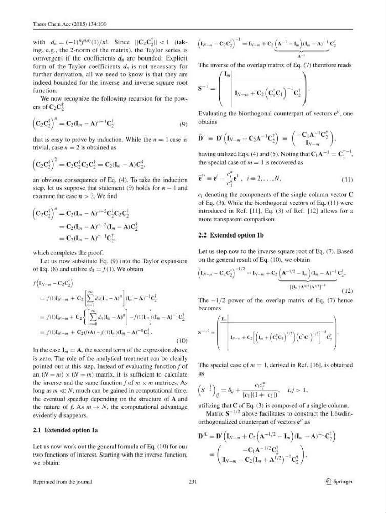
We now recognize the following recursion for the powers of C 2 C
†
2
that is easy to prove by induction. While the n = 1 case is
trivial, case n = 2 is obtained as
an obvious consequence of Eq. ( 4 ). To take the induction
step, let us suppose that statement ( 9 ) holds for n − 1 and
examine the case n > 2 . We fi nd
which completes the proof.
Let us now substitute Eq. ( 9 ) into the Taylor expansion
of Eq. ( 8 ) and utilize d 0 = f (1) . We obtain
In the case I m = A, the second term of the expression above
is zero. The role of the analytical treatment can be clearly
pointed out at this step. Instead of evaluating function f of
an (N − m) × (N − m) matrix, it is suffi cient to calculate
the inverse and the same function f of m × m matrices. As
long as m N , much can be gained in computational time,
the eventual speedup depending on the structure of A and
the nature of f . As m → N , the computational advantage
evidently disappears.
2.1 Extended option 1a
Let us now work out the general formula of Eq. ( 10 ) for our
two functions of interest. Starting with the inverse function,
we obtain:
(9)
C 2 C
†
2
n = C 2 (I m − A)
n−1 C
†
2
C 2 C
†
2
2 = C 2 C
†
2 C 2 C
†
2 = C 2 (I m − A)C
†
2 ,
C 2 C
†
2
n = C 2 (I m − A)
n−2 C
†
2 C 2 C
†
2
= C 2 (I m − A)
n−2
(I m − A)C
†
2
= C 2 (I m − A)
n−1 C
†
2 ,
(10)
f
I N−m − C 2 C
†
2
= f (1)I N−m + C 2
∞
n=1
d n (I m − A) n
(I m − A) −1 C
†
2
= f (1)I N−m + C 2
∞
n=0
d n (I m − A) n
− f (1)I m
(I m − A) −1 C
†
2
= f (1)I N−m + C 2 (f (A) − f (1)I m )(I m − A) −1 C
†
2 .
The inverse of the overlap matrix of Eq. ( 7 ) therefore reads
Evaluating the biorthogonal counterpart of vectors e i , one
obtains
having utilized Eqs. ( 4 ) and ( 5 ). Noting that C 1 A −1 = C
†−1
1 ,
the special case of m = 1 is recovered as
c i denoting the components of the single column vector C
of Eq. ( 3 ). While the biorthogonal vectors of Eq. ( 11 ) were
introduced in Ref. [ 11 ], Eq. ( 3 ) of Ref. [ 12 ] allows for a
more transparent comparison.
2.2 Extended option 1b
Let us step now to the inverse square root of Eq. ( 7 ). Based
on the general result of Eq. ( 10 ), we obtain
The −1/2 power of the overlap matrix of Eq. ( 7 ) hence
becomes
The special case of m = 1 , derived in Ref. [ 16 ], is obtained
as
utilizing that C of Eq. ( 3 ) is composed of a single column.
Matrix S −1/2 above facilitates to construct the Löwdinorthogonalized counterpart of vectors e i as
I N−m − C 2 C
†
2
−1 = I N−m + C 2
A
−1 − I m
(I m − A)
−1
훀훀
훀
A −1
C
†
2
S
−1
=
⎛
⎜
⎜
⎜
⎝
I m
I N−m + C 2
C
†
1 C 1
−1
C
†
2
⎞
⎟
⎟
⎟
⎠
.
D
= D
I N−m + C 2 A
−1 C
†
2
=
−C 1 A −1 C
†
2
I N−m
,
(11)
e
i
= e
i
−
c ∗
i
c ∗
1
e
1 , i = 2, . . . , N,
(12)
I N−m − C 2 C
†
2
−1/2 = I N−m + C 2
A
−1/2 − I m
(I m − A)
−1
[(Im+A 1/2 )A 1/2 ]
−1
C
†
2 .
S
−1/2 =
⎛
⎜
⎜
⎜
⎜
⎜
⎜
⎝
I m
I N−m + C 2
I m +
C
†
1 C 1
1/2
C
†
1 C 1
1/2
−1
C
†
2
⎞
⎟
⎟
⎟
⎟
⎟
⎟
⎠
.
S
−
1
2
ij
= δ ij +
c i c ∗
j
|c 1 |(1 + |c 1 |)
, i, j > 1,
D
L
= D
I N−m + C 2
A
−1/2
− I m
(I m − A)
−1 C
†
2
=
−C 1 A −1/2 C
†
2
I N−m − C 2
I m + A 1/2 −1 C
†
2
,
231
Reprinted from the journal
1 3
with d n = (−1) n f (n) (1)/n! . Since ||C 2 C
†
2 || < 1 (taking, e.g., the 2-norm of the matrix), the Taylor series is
convergent if the coefficients d n are bounded. Explicit
form of the Taylor coefficients d n is not necessary for
further derivation, all we need to know is that they are
indeed bounded for the inverse and inverse square root
function.
We now recognize the following recursion for the powers of C 2 C
†
2
that is easy to prove by induction. While the n = 1 case is
trivial, case n = 2 is obtained as
an obvious consequence of Eq. ( 4 ). To take the induction
step, let us suppose that statement ( 9 ) holds for n − 1 and
examine the case n > 2 . We fi nd
which completes the proof.
Let us now substitute Eq. ( 9 ) into the Taylor expansion
of Eq. ( 8 ) and utilize d 0 = f (1) . We obtain
In the case I m = A, the second term of the expression above
is zero. The role of the analytical treatment can be clearly
pointed out at this step. Instead of evaluating function f of
an (N − m) × (N − m) matrix, it is suffi cient to calculate
the inverse and the same function f of m × m matrices. As
long as m N , much can be gained in computational time,
the eventual speedup depending on the structure of A and
the nature of f . As m → N , the computational advantage
evidently disappears.
2.1 Extended option 1a
Let us now work out the general formula of Eq. ( 10 ) for our
two functions of interest. Starting with the inverse function,
we obtain:
(9)
C 2 C
†
2
n = C 2 (I m − A)
n−1 C
†
2
C 2 C
†
2
2 = C 2 C
†
2 C 2 C
†
2 = C 2 (I m − A)C
†
2 ,
C 2 C
†
2
n = C 2 (I m − A)
n−2 C
†
2 C 2 C
†
2
= C 2 (I m − A)
n−2
(I m − A)C
†
2
= C 2 (I m − A)
n−1 C
†
2 ,
(10)
f
I N−m − C 2 C
†
2
= f (1)I N−m + C 2
∞
n=1
d n (I m − A) n
(I m − A) −1 C
†
2
= f (1)I N−m + C 2
∞
n=0
d n (I m − A) n
− f (1)I m
(I m − A) −1 C
†
2
= f (1)I N−m + C 2 (f (A) − f (1)I m )(I m − A) −1 C
†
2 .
The inverse of the overlap matrix of Eq. ( 7 ) therefore reads
Evaluating the biorthogonal counterpart of vectors e i , one
obtains
having utilized Eqs. ( 4 ) and ( 5 ). Noting that C 1 A −1 = C
†−1
1 ,
the special case of m = 1 is recovered as
c i denoting the components of the single column vector C
of Eq. ( 3 ). While the biorthogonal vectors of Eq. ( 11 ) were
introduced in Ref. [ 11 ], Eq. ( 3 ) of Ref. [ 12 ] allows for a
more transparent comparison.
2.2 Extended option 1b
Let us step now to the inverse square root of Eq. ( 7 ). Based
on the general result of Eq. ( 10 ), we obtain
The −1/2 power of the overlap matrix of Eq. ( 7 ) hence
becomes
The special case of m = 1 , derived in Ref. [ 16 ], is obtained
as
utilizing that C of Eq. ( 3 ) is composed of a single column.
Matrix S −1/2 above facilitates to construct the Löwdinorthogonalized counterpart of vectors e i as
I N−m − C 2 C
†
2
−1 = I N−m + C 2
A
−1 − I m
(I m − A)
−1
훀훀
훀
A −1
C
†
2
S
−1
=
⎛
⎜
⎜
⎜
⎝
I m
I N−m + C 2
C
†
1 C 1
−1
C
†
2
⎞
⎟
⎟
⎟
⎠
.
D
= D
I N−m + C 2 A
−1 C
†
2
=
−C 1 A −1 C
†
2
I N−m
,
(11)
e
i
= e
i
−
c ∗
i
c ∗
1
e
1 , i = 2, . . . , N,
(12)
I N−m − C 2 C
†
2
−1/2 = I N−m + C 2
A
−1/2 − I m
(I m − A)
−1
[(Im+A 1/2 )A 1/2 ]
−1
C
†
2 .
S
−1/2 =
⎛
⎜
⎜
⎜
⎜
⎜
⎜
⎝
I m
I N−m + C 2
I m +
C
†
1 C 1
1/2
C
†
1 C 1
1/2
−1
C
†
2
⎞
⎟
⎟
⎟
⎟
⎟
⎟
⎠
.
S
−
1
2
ij
= δ ij +
c i c ∗
j
|c 1 |(1 + |c 1 |)
, i, j > 1,
D
L
= D
I N−m + C 2
A
−1/2
− I m
(I m − A)
−1 C
†
2
=
−C 1 A −1/2 C
†
2
I N−m − C 2
I m + A 1/2 −1 C
†
2
,
231
Reprinted from the journal