

Theor Chem Acc (2015) 134:118
1 3
in turn implies that the corresponding coeffi cient c p is, in
general, greater than zero. At fi rst sight, the expression for
the energy ( 10 ) looks identical to its APSG counterpart, but
one should keep in mind that orbitals in GVB-PP are paired
[cf. Eq. ( 4 )] and the set of conditions given in Eq. ( 9 ) must
be imposed while optimizing the functional ( 10 ). Clearly
therefore, the APSG energy is a lower bound to the GVBPP energy and both are bounded from below by the exact
ground-state value,
There is one signifi cant computational advantage of optimizing the GVB-PP energy functional rather than that of
the APSG. In the latter, all natural orbitals have nonzero
occupation numbers, whereas in the former, only N orbitals are fractionally occupied and the rest of orbitals forms
a set of virtual (unoccupied) orbitals. A need to optimize
all (often very weakly occupied) orbitals in the APSG
approach leads to a slowly converging optimization problem. Optimization of the GVB-PP energy, on the other
hand, is much more effi cient (orbitals which are very
weakly occupied in APSG are virtual orbitals in GVB and
have no contribution to the energy).
GVB-PP method has been applied mostly to description
of ground states of molecules although, in principle, one
can also converge the GVB-PP energy to a selected excited
state. A time-dependent linear response theory approach,
which allows one to fi nd a number of excitation energies
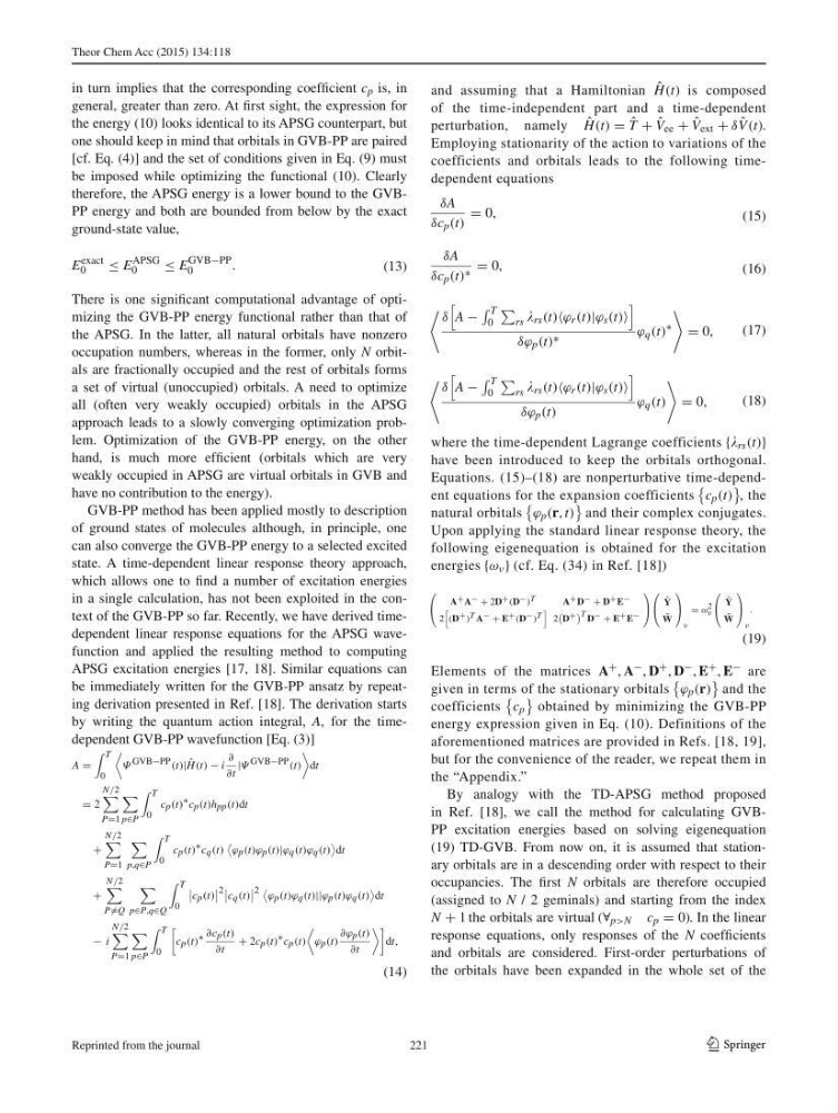
in a single calculation, has not been exploited in the context of the GVB-PP so far. Recently, we have derived timedependent linear response equations for the APSG wavefunction and applied the resulting method to computing
APSG excitation energies [ 17 , 18 ]. Similar equations can
be immediately written for the GVB-PP ansatz by repeating derivation presented in Ref. [ 18 ]. The derivation starts
by writing the quantum action integral, A , for the timedependent GVB-PP wavefunction [Eq. ( 3 )]
(13)
E
exact
0
≤ E
APSG
0
≤ E
GVB−PP
0
.
(14)
A =
T
0
Ψ GVB−PP (t)| ˆ
H(t) − i
∂
∂t
|Ψ GVB−PP (t)
dt
= 2
N/2
P=1
p∈P
T
0
c p (t) ∗ c p (t)h pp (t)dt
+
N/2
P=1
p,q∈P
T
0
c p (t) ∗ c q (t)
ϕ p (t)ϕ p (t)|ϕ q (t)ϕ q (t)
dt
+
N/2
P =Q
p∈P,q∈Q
T
0
c p (t)
2
c q (t)
2
ϕ p (t)ϕ q (t)||ϕ p (t)ϕ q (t)
dt
− i
N/2
P=1
p∈P
T
0
c p (t) ∗ ∂c p (t)
∂t
+ 2c p (t) ∗ c p (t)
ϕ p (t)
∂ϕ p (t)
∂t
dt,
and assuming that a Hamiltonian ˆ
H(t) is composed
of the time-independent part and a time-dependent
perturbation, namely ˆ
H(t) = ˆ
T + ˆ
V ee + ˆ
V ext + δ ˆ
V (t) .
Employing stationarity of the action to variations of the
coefficients and orbitals leads to the following timedependent equations
where the time-dependent Lagrange coefficients { rs (t)}
have been introduced to keep the orbitals orthogonal.
Equations. ( 15 )–( 18 ) are nonperturbative time-dependent equations for the expansion coefficients
c p (t)
, the
natural orbitals
ϕ p (r, t)
and their complex conjugates.
Upon applying the standard linear response theory, the
following eigenequation is obtained for the excitation
energies {ω ν } (cf. Eq. ( 34 ) in Ref. [ 18 ])
Elements of the matrices A + , A − , D + , D − , E + , E − are
given in terms of the stationary orbitals
ϕ p (r)
and the
coefficients
c p
obtained by minimizing the GVB-PP
energy expression given in Eq. ( 10 ). Definitions of the
aforementioned matrices are provided in Refs. [ 18 , 19 ],
but for the convenience of the reader, we repeat them in
the “ Appendix .”
By analogy with the TD-APSG method proposed
in Ref. [ 18 ], we call the method for calculating GVBPP excitation energies based on solving eigenequation
( 19 ) TD-GVB. From now on, it is assumed that stationary orbitals are in a descending order with respect to their
occupancies. The fi rst N orbitals are therefore occupied
(assigned to N / 2 geminals) and starting from the index
N + 1 the orbitals are virtual (∀ p>N c p = 0) . In the linear
response equations, only responses of the N coeffi cients
and orbitals are considered. First-order perturbations of
the orbitals have been expanded in the whole set of the
(15)
δA
δc p (t)
= 0,
(16)
δA
δc p (t) ∗ = 0,
(17)
δ
A −
T
0
rs rs (t)ϕ r (t)|ϕ s (t)
δϕ p (t) ∗
ϕ q (t)
∗
= 0,
(18)
δ
A −
T
0
rs rs (t)ϕ r (t)|ϕ s (t)
δϕ p (t)
ϕ q (t)
= 0,
(19)
⎛
⎝
A + A − + 2D + (D − ) T
A + D − + D + E −
2
(D + ) T A − + E + (D − ) T
2
D + T D − + E + E −
⎞
⎠
⎛
⎝
˜
Y
˜
W
⎞
⎠
ν
= ω 2
ν
⎛
⎝
˜
Y
˜
W
⎞
⎠
ν
.
221
Reprinted from the journal
1 3
in turn implies that the corresponding coeffi cient c p is, in
general, greater than zero. At fi rst sight, the expression for
the energy ( 10 ) looks identical to its APSG counterpart, but
one should keep in mind that orbitals in GVB-PP are paired
[cf. Eq. ( 4 )] and the set of conditions given in Eq. ( 9 ) must
be imposed while optimizing the functional ( 10 ). Clearly
therefore, the APSG energy is a lower bound to the GVBPP energy and both are bounded from below by the exact
ground-state value,
There is one signifi cant computational advantage of optimizing the GVB-PP energy functional rather than that of
the APSG. In the latter, all natural orbitals have nonzero
occupation numbers, whereas in the former, only N orbitals are fractionally occupied and the rest of orbitals forms
a set of virtual (unoccupied) orbitals. A need to optimize
all (often very weakly occupied) orbitals in the APSG
approach leads to a slowly converging optimization problem. Optimization of the GVB-PP energy, on the other
hand, is much more effi cient (orbitals which are very
weakly occupied in APSG are virtual orbitals in GVB and
have no contribution to the energy).
GVB-PP method has been applied mostly to description
of ground states of molecules although, in principle, one
can also converge the GVB-PP energy to a selected excited
state. A time-dependent linear response theory approach,
which allows one to fi nd a number of excitation energies
in a single calculation, has not been exploited in the context of the GVB-PP so far. Recently, we have derived timedependent linear response equations for the APSG wavefunction and applied the resulting method to computing
APSG excitation energies [ 17 , 18 ]. Similar equations can
be immediately written for the GVB-PP ansatz by repeating derivation presented in Ref. [ 18 ]. The derivation starts
by writing the quantum action integral, A , for the timedependent GVB-PP wavefunction [Eq. ( 3 )]
(13)
E
exact
0
≤ E
APSG
0
≤ E
GVB−PP
0
.
(14)
A =
T
0
Ψ GVB−PP (t)| ˆ
H(t) − i
∂
∂t
|Ψ GVB−PP (t)
dt
= 2
N/2
P=1
p∈P
T
0
c p (t) ∗ c p (t)h pp (t)dt
+
N/2
P=1
p,q∈P
T
0
c p (t) ∗ c q (t)
ϕ p (t)ϕ p (t)|ϕ q (t)ϕ q (t)
dt
+
N/2
P =Q
p∈P,q∈Q
T
0
c p (t)
2
c q (t)
2
ϕ p (t)ϕ q (t)||ϕ p (t)ϕ q (t)
dt
− i
N/2
P=1
p∈P
T
0
c p (t) ∗ ∂c p (t)
∂t
+ 2c p (t) ∗ c p (t)
ϕ p (t)
∂ϕ p (t)
∂t
dt,
and assuming that a Hamiltonian ˆ
H(t) is composed
of the time-independent part and a time-dependent
perturbation, namely ˆ
H(t) = ˆ
T + ˆ
V ee + ˆ
V ext + δ ˆ
V (t) .
Employing stationarity of the action to variations of the
coefficients and orbitals leads to the following timedependent equations
where the time-dependent Lagrange coefficients { rs (t)}
have been introduced to keep the orbitals orthogonal.
Equations. ( 15 )–( 18 ) are nonperturbative time-dependent equations for the expansion coefficients
c p (t)
, the
natural orbitals
ϕ p (r, t)
and their complex conjugates.
Upon applying the standard linear response theory, the
following eigenequation is obtained for the excitation
energies {ω ν } (cf. Eq. ( 34 ) in Ref. [ 18 ])
Elements of the matrices A + , A − , D + , D − , E + , E − are
given in terms of the stationary orbitals
ϕ p (r)
and the
coefficients
c p
obtained by minimizing the GVB-PP
energy expression given in Eq. ( 10 ). Definitions of the
aforementioned matrices are provided in Refs. [ 18 , 19 ],
but for the convenience of the reader, we repeat them in
the “ Appendix .”
By analogy with the TD-APSG method proposed
in Ref. [ 18 ], we call the method for calculating GVBPP excitation energies based on solving eigenequation
( 19 ) TD-GVB. From now on, it is assumed that stationary orbitals are in a descending order with respect to their
occupancies. The fi rst N orbitals are therefore occupied
(assigned to N / 2 geminals) and starting from the index
N + 1 the orbitals are virtual (∀ p>N c p = 0) . In the linear
response equations, only responses of the N coeffi cients
and orbitals are considered. First-order perturbations of
the orbitals have been expanded in the whole set of the
(15)
δA
δc p (t)
= 0,
(16)
δA
δc p (t) ∗ = 0,
(17)
δ
A −
T
0
rs rs (t)ϕ r (t)|ϕ s (t)
δϕ p (t) ∗
ϕ q (t)
∗
= 0,
(18)
δ
A −
T
0
rs rs (t)ϕ r (t)|ϕ s (t)
δϕ p (t)
ϕ q (t)
= 0,
(19)
⎛
⎝
A + A − + 2D + (D − ) T
A + D − + D + E −
2
(D + ) T A − + E + (D − ) T
2
D + T D − + E + E −
⎞
⎠
⎛
⎝
˜
Y
˜
W
⎞
⎠
ν
= ω 2
ν
⎛
⎝
˜
Y
˜
W
⎞
⎠
ν
.
221
Reprinted from the journal