

Theor Chem Acc (2015) 134:118
1 3
Interestingly, recently the GVB-PP approximation has been
reinvented within the natural orbital functional theory [ 11 ,
12 ]. Namely, one of the recently proposed natural orbital
functionals—PNOF5 [ 13 ]—obtained by reconstructing
two-electron reduced density matrix in terms of the oneelectron reduced density matrix, has been shown to be
equivalent to the GVB-PP approximation [ 14 ]. Fully variational PNOF5 calculations have proved usefulness of the
method in predicting ground-state energies of molecules of
diverse and challenging electronic structures [ 13 , 15 ].
GVB or GVB-PP approximations have been mostly
employed to describe ground states of molecules. However,
since the methods are variational and they are based on a
wavefunction ansatz, then excited states calculations should
be also possible in a similar fashion as it is done for the multiconfi guration self-consistent fi eld methods. However, application of the GVB-PP method to excited states either by
performing variational calculations or by employing the timedependent linear response formalism has not been explored
so far. The aim of this paper is to fi ll this gap. We present a
linear response GVB-PP formalism leading to obtaining singlet excitation energies and discuss its performance by presenting excitation energy curves for a few small molecules.
2 Theory
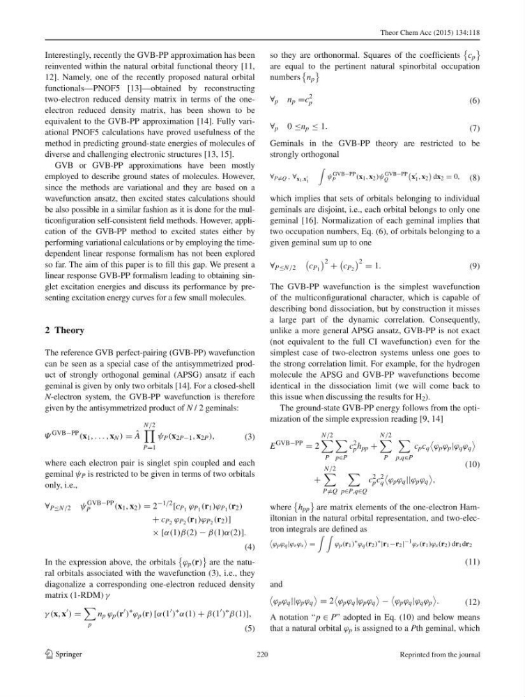
The reference GVB perfect-pairing (GVB-PP) wavefunction
can be seen as a special case of the antisymmetrized product of strongly orthogonal geminal (APSG) ansatz if each
geminal is given by only two orbitals [ 14 ]. For a closed-shell
N -electron system, the GVB-PP wavefunction is therefore
given by the antisymmetrized product of N / 2 geminals:
where each electron pair is singlet spin coupled and each
geminal ψ P is restricted to be given in terms of two orbitals
only, i.e.,
In the expression above, the orbitals
ϕ p (r)
are the natural orbitals associated with the wavefunction ( 3 ), i.e., they
diagonalize a corresponding one-electron reduced density
matrix (1-RDM) γ
(3)
Ψ
GVB−PP
(x 1 , . . . , x N ) = ˆ
A
N/2
P=1
ψ P (x 2P−1 , x 2P ),
(4)
∀ P≤N/2 ψ
GVB−PP
P
(x 1 , x 2 ) = 2
−1/2
[c P 1 ϕ P 1 (r 1 )ϕ P 1 (r 2 )
+ c P 2 ϕ P 2 (r 1 )ϕ P 2 (r 2 )]
× [α(1)β(2) − β(1)α(2)].
(5)
γ (x, x
) =
p
n p ϕ p (r
)
∗
ϕ p (r) [α(1
)
∗
α(1) + β(1
)
∗
β(1)],
so they are orthonormal. Squares of the coeffi cients
c p
are equal to the pertinent natural spinorbital occupation
numbers
n p
Geminals in the GVB-PP theory are restricted to be
strongly orthogonal
which implies that sets of orbitals belonging to individual
geminals are disjoint, i.e., each orbital belongs to only one
geminal [ 16 ]. Normalization of each geminal implies that
two occupation numbers, Eq. ( 6 ), of orbitals belonging to a
given geminal sum up to one
The GVB-PP wavefunction is the simplest wavefunction
of the multiconfi gurational character, which is capable of
describing bond dissociation, but by construction it misses
a large part of the dynamic correlation. Consequently,
unlike a more general APSG ansatz, GVB-PP is not exact
(not equivalent to the full CI wavefunction) even for the
simplest case of two-electron systems unless one goes to
the strong correlation limit. For example, for the hydrogen
molecule the APSG and GVB-PP wavefunctions become
identical in the dissociation limit (we will come back to
this issue when discussing the results for H 2 ).
The ground-state GVB-PP energy follows from the optimization of the simple expression reading [ 9 , 14 ]
where
h pp
are matrix elements of the one-electron Hamiltonian in the natural orbital representation, and two-electron integrals are defi ned as
and
A notation “ p ∈ P ” adopted in Eq. ( 10 ) and below means
that a natural orbital ϕ p is assigned to a P th geminal, which
(6)
∀ p n p =c
2
p
(7)
∀ p 0 ≤n p ≤ 1.
(8)
∀ P =Q , ∀ x 1 ,x
1
ψ
GVB−PP
P
(x 1 , x 2 )ψ
GVB−PP
Q
x
1 , x 2
dx 2 = 0,
(9)
∀ P≤N/2
c P 1
2 +
c P 2
2 = 1.
(10)
E
GVB−PP
= 2
N/2
P
p∈P
c
2
p h pp +
N/2
P
p,q∈P
c p c q
ϕ p ϕ p |ϕ q ϕ q
+
N/2
P =Q
p∈P,q∈Q
c
2
p c
2
q
ϕ p ϕ q ||ϕ p ϕ q
,
(11)
ϕ p ϕ q |ϕ r ϕ s
=
ϕ p (r 1 )
∗ ϕ q (r 2 )
∗ |r 1 −r 2 |
−1 ϕ r (r 1 )ϕ s (r 2 ) dr 1 dr 2
(12)
ϕ p ϕ q ||ϕ p ϕ q
= 2
ϕ p ϕ q |ϕ p ϕ q
−
ϕ p ϕ q |ϕ q ϕ p
.
220
Reprinted from the journal
1 3
Interestingly, recently the GVB-PP approximation has been
reinvented within the natural orbital functional theory [ 11 ,
12 ]. Namely, one of the recently proposed natural orbital
functionals—PNOF5 [ 13 ]—obtained by reconstructing
two-electron reduced density matrix in terms of the oneelectron reduced density matrix, has been shown to be
equivalent to the GVB-PP approximation [ 14 ]. Fully variational PNOF5 calculations have proved usefulness of the
method in predicting ground-state energies of molecules of
diverse and challenging electronic structures [ 13 , 15 ].
GVB or GVB-PP approximations have been mostly
employed to describe ground states of molecules. However,
since the methods are variational and they are based on a
wavefunction ansatz, then excited states calculations should
be also possible in a similar fashion as it is done for the multiconfi guration self-consistent fi eld methods. However, application of the GVB-PP method to excited states either by
performing variational calculations or by employing the timedependent linear response formalism has not been explored
so far. The aim of this paper is to fi ll this gap. We present a
linear response GVB-PP formalism leading to obtaining singlet excitation energies and discuss its performance by presenting excitation energy curves for a few small molecules.
2 Theory
The reference GVB perfect-pairing (GVB-PP) wavefunction
can be seen as a special case of the antisymmetrized product of strongly orthogonal geminal (APSG) ansatz if each
geminal is given by only two orbitals [ 14 ]. For a closed-shell
N -electron system, the GVB-PP wavefunction is therefore
given by the antisymmetrized product of N / 2 geminals:
where each electron pair is singlet spin coupled and each
geminal ψ P is restricted to be given in terms of two orbitals
only, i.e.,
In the expression above, the orbitals
ϕ p (r)
are the natural orbitals associated with the wavefunction ( 3 ), i.e., they
diagonalize a corresponding one-electron reduced density
matrix (1-RDM) γ
(3)
Ψ
GVB−PP
(x 1 , . . . , x N ) = ˆ
A
N/2
P=1
ψ P (x 2P−1 , x 2P ),
(4)
∀ P≤N/2 ψ
GVB−PP
P
(x 1 , x 2 ) = 2
−1/2
[c P 1 ϕ P 1 (r 1 )ϕ P 1 (r 2 )
+ c P 2 ϕ P 2 (r 1 )ϕ P 2 (r 2 )]
× [α(1)β(2) − β(1)α(2)].
(5)
γ (x, x
) =
p
n p ϕ p (r
)
∗
ϕ p (r) [α(1
)
∗
α(1) + β(1
)
∗
β(1)],
so they are orthonormal. Squares of the coeffi cients
c p
are equal to the pertinent natural spinorbital occupation
numbers
n p
Geminals in the GVB-PP theory are restricted to be
strongly orthogonal
which implies that sets of orbitals belonging to individual
geminals are disjoint, i.e., each orbital belongs to only one
geminal [ 16 ]. Normalization of each geminal implies that
two occupation numbers, Eq. ( 6 ), of orbitals belonging to a
given geminal sum up to one
The GVB-PP wavefunction is the simplest wavefunction
of the multiconfi gurational character, which is capable of
describing bond dissociation, but by construction it misses
a large part of the dynamic correlation. Consequently,
unlike a more general APSG ansatz, GVB-PP is not exact
(not equivalent to the full CI wavefunction) even for the
simplest case of two-electron systems unless one goes to
the strong correlation limit. For example, for the hydrogen
molecule the APSG and GVB-PP wavefunctions become
identical in the dissociation limit (we will come back to
this issue when discussing the results for H 2 ).
The ground-state GVB-PP energy follows from the optimization of the simple expression reading [ 9 , 14 ]
where
h pp
are matrix elements of the one-electron Hamiltonian in the natural orbital representation, and two-electron integrals are defi ned as
and
A notation “ p ∈ P ” adopted in Eq. ( 10 ) and below means
that a natural orbital ϕ p is assigned to a P th geminal, which
(6)
∀ p n p =c
2
p
(7)
∀ p 0 ≤n p ≤ 1.
(8)
∀ P =Q , ∀ x 1 ,x
1
ψ
GVB−PP
P
(x 1 , x 2 )ψ
GVB−PP
Q
x
1 , x 2
dx 2 = 0,
(9)
∀ P≤N/2
c P 1
2 +
c P 2
2 = 1.
(10)
E
GVB−PP
= 2
N/2
P
p∈P
c
2
p h pp +
N/2
P
p,q∈P
c p c q
ϕ p ϕ p |ϕ q ϕ q
+
N/2
P =Q
p∈P,q∈Q
c
2
p c
2
q
ϕ p ϕ q ||ϕ p ϕ q
,
(11)
ϕ p ϕ q |ϕ r ϕ s
=
ϕ p (r 1 )
∗ ϕ q (r 2 )
∗ |r 1 −r 2 |
−1 ϕ r (r 1 )ϕ s (r 2 ) dr 1 dr 2
(12)
ϕ p ϕ q ||ϕ p ϕ q
= 2
ϕ p ϕ q |ϕ p ϕ q
−
ϕ p ϕ q |ϕ q ϕ p
.
220
Reprinted from the journal