

Theor Chem Acc (2016) 135:3
1 3
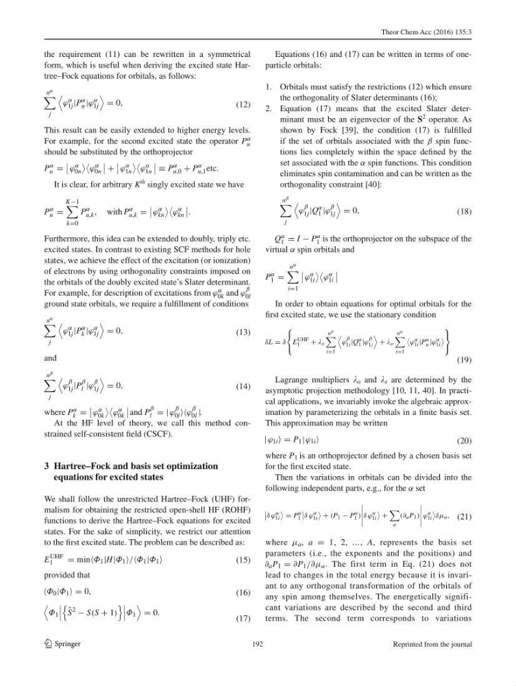
the requirement ( 11 ) can be rewritten in a symmetrical
form, which is useful when deriving the excited state Hartree–Fock equations for orbitals, as follows:
This result can be easily extended to higher energy levels.
For example, for the second excited state the operator P α
u
should be substituted by the orthoprojector
It is clear, for arbitrary K
th singly excited state we have
Furthermore, this idea can be extended to doubly, triply etc.
excited states. In contrast to existing SCF methods for hole
states, we achieve the effect of the excitation (or ionization)
of electrons by using orthogonality constraints imposed on
the orbitals of the doubly excited state’s Slater determinant.
For example, for description of excitations from ϕ α
0k and ϕ
β
0l
ground state orbitals, we require a fulfi llment of conditions
and
where P α
k =
ϕ α
0k
ϕ α
0k
and P
β
l = |ϕ
β
0l ϕ
β
0l | .
At the HF level of theory, we call this method constrained self-consistent fi eld (CSCF).
3 Hartree–Fock and basis set optimization
equations for excited states
We shall follow the unrestricted Hartree–Fock (UHF) formalism for obtaining the restricted open-shell HF (ROHF)
functions to derive the Hartree–Fock equations for excited
states. For the sake of simplicity, we restrict our attention
to the fi rst excited state. The problem can be described as:
provided that
(12)
n α
j
ϕ
α
1j |P
α
u |ϕ
α
1j
= 0,
P
α
u =
ϕ
α
0n
ϕ
α
0n
횿 +
ϕ
α
1n
ϕ
α
1n
≡ P
α
u,0 + P
α
u,1 etc.
P
α
u =
K−1
k=0
P
α
u,k , with P
α
u,k =
ϕ
α
kn
ϕ
α
kn
.
(13)
n α
j
ϕ
α
1j |P
α
k |ϕ
α
1j
= 0,
(14)
n β
j
ϕ
β
1j |P
β
l |ϕ
β
1j
= 0,
(15)
E
UHF
1
= minΦ 1 |H|Φ 1 /Φ 1 |Φ 1
(16)
Φ 0 |Φ 1 = 0,
(17)
Φ 1
ˆ
S
2
− S(S + 1)
Φ1
= 0.
Equations ( 16 ) and ( 17 ) can be written in terms of oneparticle orbitals:
1. Orbitals must satisfy the restrictions ( 12 ) which ensure
the orthogonality of Slater determinants ( 16 );
2. Equation ( 17 ) means that the excited Slater determinant must be an eigenvector of the S
2 operator. As
shown by Fock [ 39 ], the condition ( 17 ) is fulfi lled
if the set of orbitals associated with the β spin functions lies completely within the space defi ned by the
set associated with the α spin functions. This condition
eliminates spin contamination and can be written as the
orthogonality constraint [ 40 ]:
Q α
1 = I − P α
1 is the orthoprojector on the subspace of the
virtual α spin orbitals and
In order to obtain equations for optimal orbitals for the
fi rst excited state, we use the stationary condition
Lagrange multipliers o and s are determined by the
asymptotic projection methodology [ 10 , 11 , 40 ]. In practical applications, we invariably invoke the algebraic approximation by parameterizing the orbitals in a fi nite basis set.
This approximation may be written
where P 1 is an orthoprojector defi ned by a chosen basis set
for the fi rst excited state.
Then the variations in orbitals can be divided into the
following independent parts, e.g., for the α set
where μ a , a = 1, 2, … , A , represents the basis set
parameters (i.e., the exponents and the positions) and
∂ a P 1 = ∂P 1 /∂μ a . The first term in Eq. ( 21 ) does not
lead to changes in the total energy because it is invariant to any orthogonal transformation of the orbitals of
any spin among themselves. The energetically significant variations are described by the second and third
terms. The second term corresponds to variations
(18)
n β
j
ϕ
β
1j |Q
α
1 |ϕ
β
1j
= 0,
P
α
1 =
n α
i=1
ϕ
α
1i
ϕ
α
1i
(19)
δL = δ
⎧
⎨
⎩
E
UHF
1
+ s
n β
i=1
ϕ
β
1i |Q
α
1 |ϕ
β
1i
+ o
n α
i=1
ϕ
α
1i |P
α
u |ϕ
α
1i
⎫
⎬
⎭
(20)
| ϕ 1i = P 1 | ϕ 1i
(21)
δ ϕ
α
1i
= P
α
1
δ ϕ
α
1i
+ (P 1 − P
α
1 )
δ ϕ
α
1i
+
a
(∂ a P 1 )
ϕ
α
1i
δμ a ,
192
Reprinted from the journal
1 3
the requirement ( 11 ) can be rewritten in a symmetrical
form, which is useful when deriving the excited state Hartree–Fock equations for orbitals, as follows:
This result can be easily extended to higher energy levels.
For example, for the second excited state the operator P α
u
should be substituted by the orthoprojector
It is clear, for arbitrary K
th singly excited state we have
Furthermore, this idea can be extended to doubly, triply etc.
excited states. In contrast to existing SCF methods for hole
states, we achieve the effect of the excitation (or ionization)
of electrons by using orthogonality constraints imposed on
the orbitals of the doubly excited state’s Slater determinant.
For example, for description of excitations from ϕ α
0k and ϕ
β
0l
ground state orbitals, we require a fulfi llment of conditions
and
where P α
k =
ϕ α
0k
ϕ α
0k
and P
β
l = |ϕ
β
0l ϕ
β
0l | .
At the HF level of theory, we call this method constrained self-consistent fi eld (CSCF).
3 Hartree–Fock and basis set optimization
equations for excited states
We shall follow the unrestricted Hartree–Fock (UHF) formalism for obtaining the restricted open-shell HF (ROHF)
functions to derive the Hartree–Fock equations for excited
states. For the sake of simplicity, we restrict our attention
to the fi rst excited state. The problem can be described as:
provided that
(12)
n α
j
ϕ
α
1j |P
α
u |ϕ
α
1j
= 0,
P
α
u =
ϕ
α
0n
ϕ
α
0n
횿 +
ϕ
α
1n
ϕ
α
1n
≡ P
α
u,0 + P
α
u,1 etc.
P
α
u =
K−1
k=0
P
α
u,k , with P
α
u,k =
ϕ
α
kn
ϕ
α
kn
.
(13)
n α
j
ϕ
α
1j |P
α
k |ϕ
α
1j
= 0,
(14)
n β
j
ϕ
β
1j |P
β
l |ϕ
β
1j
= 0,
(15)
E
UHF
1
= minΦ 1 |H|Φ 1 /Φ 1 |Φ 1
(16)
Φ 0 |Φ 1 = 0,
(17)
Φ 1
ˆ
S
2
− S(S + 1)
Φ1
= 0.
Equations ( 16 ) and ( 17 ) can be written in terms of oneparticle orbitals:
1. Orbitals must satisfy the restrictions ( 12 ) which ensure
the orthogonality of Slater determinants ( 16 );
2. Equation ( 17 ) means that the excited Slater determinant must be an eigenvector of the S
2 operator. As
shown by Fock [ 39 ], the condition ( 17 ) is fulfi lled
if the set of orbitals associated with the β spin functions lies completely within the space defi ned by the
set associated with the α spin functions. This condition
eliminates spin contamination and can be written as the
orthogonality constraint [ 40 ]:
Q α
1 = I − P α
1 is the orthoprojector on the subspace of the
virtual α spin orbitals and
In order to obtain equations for optimal orbitals for the
fi rst excited state, we use the stationary condition
Lagrange multipliers o and s are determined by the
asymptotic projection methodology [ 10 , 11 , 40 ]. In practical applications, we invariably invoke the algebraic approximation by parameterizing the orbitals in a fi nite basis set.
This approximation may be written
where P 1 is an orthoprojector defi ned by a chosen basis set
for the fi rst excited state.
Then the variations in orbitals can be divided into the
following independent parts, e.g., for the α set
where μ a , a = 1, 2, … , A , represents the basis set
parameters (i.e., the exponents and the positions) and
∂ a P 1 = ∂P 1 /∂μ a . The first term in Eq. ( 21 ) does not
lead to changes in the total energy because it is invariant to any orthogonal transformation of the orbitals of
any spin among themselves. The energetically significant variations are described by the second and third
terms. The second term corresponds to variations
(18)
n β
j
ϕ
β
1j |Q
α
1 |ϕ
β
1j
= 0,
P
α
1 =
n α
i=1
ϕ
α
1i
ϕ
α
1i
(19)
δL = δ
⎧
⎨
⎩
E
UHF
1
+ s
n β
i=1
ϕ
β
1i |Q
α
1 |ϕ
β
1i
+ o
n α
i=1
ϕ
α
1i |P
α
u |ϕ
α
1i
⎫
⎬
⎭
(20)
| ϕ 1i = P 1 | ϕ 1i
(21)
δ ϕ
α
1i
= P
α
1
δ ϕ
α
1i
+ (P 1 − P
α
1 )
δ ϕ
α
1i
+
a
(∂ a P 1 )
ϕ
α
1i
δμ a ,
192
Reprinted from the journal