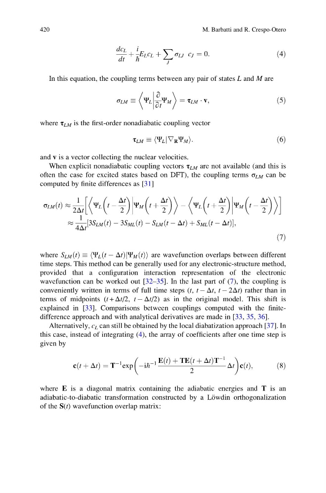
dc L
dt
þ
i
h
E L c L þ
X
J
σ LJ c J ¼ 0:
ð4Þ
In this equation, the coupling terms between any pair of states L and M are
σ LM Ψ L
∂
∂t
Ψ M
(
)
¼ τ LM Á v;
ð5Þ
where τ LM is the first-order nonadiabatic coupling vector
τ LM Ψ L ∇ R Ψ M
j
h
i :
ð6Þ
and v is a vector collecting the nuclear velocities.
When explicit nonadiabatic coupling vectors τ LM are not available (and this is
often the case for excited states based on DFT), the coupling terms σ LM can be
computed by finite differences as [31]
σ LM t
ð Þ %
1
2Δt
Ψ L t À
Δt
2
Ψ M t þ
Δt
2
(
)
À Ψ L t þ
Δt
2
Ψ M t À
Δt
2
(
) !
%
1
4Δt
3S LM t
ð Þ À 3S ML t
ð Þ À S LM t À Δt
ð
ÞþS ML t À Δt
ð
Þ
½
Š ;
ð7Þ
where S LM t
ð Þ Ψ L t À Δt
ð
ÞΨ M t
ð Þ
j
h
i are wavefunction overlaps between different
time steps. This method can be generally used for any electronic-structure method,
provided that a configuration interaction representation of the electronic
wavefunction can be worked out [32–35]. In the last part of (7), the coupling is
conveniently written in terms of full time steps (t, t À Δt, t À 2Δt) rather than in
terms of midpoints (t + Δt/2, t À Δt/2) as in the original model. This shift is
explained in [33]. Comparisons between couplings computed with the finitedifference approach and with analytical derivatives are made in [33, 35, 36].
Alternatively, c L can still be obtained by the local diabatization approach [37]. In
this case, instead of integrating (4), the array of coefficients after one time step is
given by
c t þ Δt
ð
Þ¼T
À1 exp Ài h
À1 E t
ð Þ þ TE t þ Δt
ð
ÞT
À1
2
Δt
c t
ð Þ;
ð8Þ
where E is a diagonal matrix containing the adiabatic energies and T is an
adiabatic-to-diabatic transformation constructed by a Lo ¨wdin orthogonalization
of the S(t) wavefunction overlap matrix:
420
M. Barbatti and R. Crespo-Otero