

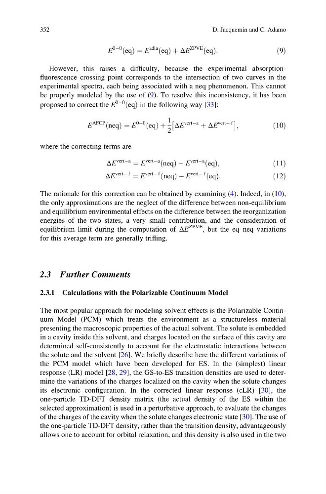
E
0À0 eq
ð Þ ¼ E
adia eq
ð Þ þ ΔE
ZPVE eq
ð Þ:
ð9Þ
However, this raises a difficulty, because the experimental absorptionfluorescence crossing point corresponds to the intersection of two curves in the
experimental spectra, each being associated with a neq phenomenon. This cannot
be properly modeled by the use of (9). To resolve this inconsistency, it has been
proposed to correct the E
0À0 eq
ð Þ in the following way [33]:
E
AFCP neq
ð Þ ¼ E
0À0 eq
ð Þ þ
1
2
ΔE
vertÀa
þ ΔE
vertÀ f
Â
à ;
ð10Þ
where the correcting terms are
ΔE
vertÀa
¼ E
vertÀa neq
ð ÞÀ E
vertÀa eq
ð Þ;
ð11Þ
ΔE
vertÀ f
¼ E
vertÀ f neq
ð ÞÀE
vertÀ f eq
ð Þ:
ð12Þ
The rationale for this correction can be obtained by examining (4). Indeed, in (10),
the only approximations are the neglect of the difference between non-equilibrium
and equilibrium environmental effects on the difference between the reorganization
energies of the two states, a very small contribution, and the consideration of
equilibrium limit during the computation of ΔE
ZPVE
, but the eq–neq variations
for this average term are generally trifling.
2.3 Further Comments
2.3.1 Calculations with the Polarizable Continuum Model
The most popular approach for modeling solvent effects is the Polarizable Continuum Model (PCM) which treats the environment as a structureless material
presenting the macroscopic properties of the actual solvent. The solute is embedded
in a cavity inside this solvent, and charges located on the surface of this cavity are
determined self-consistently to account for the electrostatic interactions between
the solute and the solvent [26]. We briefly describe here the different variations of
the PCM model which have been developed for ES. In the (simplest) linear
response (LR) model [28, 29], the GS-to-ES transition densities are used to determine the variations of the charges localized on the cavity when the solute changes
its electronic configuration. In the corrected linear response (cLR) [30], the
one-particle TD-DFT density matrix (the actual density of the ES within the
selected approximation) is used in a perturbative approach, to evaluate the changes
of the charges of the cavity when the solute changes electronic state [30]. The use of
the one-particle TD-DFT density, rather than the transition density, advantageously
allows one to account for orbital relaxation, and this density is also used in the two
352
D. Jacquemin and C. Adamo
0À0 eq
ð Þ ¼ E
adia eq
ð Þ þ ΔE
ZPVE eq
ð Þ:
ð9Þ
However, this raises a difficulty, because the experimental absorptionfluorescence crossing point corresponds to the intersection of two curves in the
experimental spectra, each being associated with a neq phenomenon. This cannot
be properly modeled by the use of (9). To resolve this inconsistency, it has been
proposed to correct the E
0À0 eq
ð Þ in the following way [33]:
E
AFCP neq
ð Þ ¼ E
0À0 eq
ð Þ þ
1
2
ΔE
vertÀa
þ ΔE
vertÀ f
Â
à ;
ð10Þ
where the correcting terms are
ΔE
vertÀa
¼ E
vertÀa neq
ð ÞÀ E
vertÀa eq
ð Þ;
ð11Þ
ΔE
vertÀ f
¼ E
vertÀ f neq
ð ÞÀE
vertÀ f eq
ð Þ:
ð12Þ
The rationale for this correction can be obtained by examining (4). Indeed, in (10),
the only approximations are the neglect of the difference between non-equilibrium
and equilibrium environmental effects on the difference between the reorganization
energies of the two states, a very small contribution, and the consideration of
equilibrium limit during the computation of ΔE
ZPVE
, but the eq–neq variations
for this average term are generally trifling.
2.3 Further Comments
2.3.1 Calculations with the Polarizable Continuum Model
The most popular approach for modeling solvent effects is the Polarizable Continuum Model (PCM) which treats the environment as a structureless material
presenting the macroscopic properties of the actual solvent. The solute is embedded
in a cavity inside this solvent, and charges located on the surface of this cavity are
determined self-consistently to account for the electrostatic interactions between
the solute and the solvent [26]. We briefly describe here the different variations of
the PCM model which have been developed for ES. In the (simplest) linear
response (LR) model [28, 29], the GS-to-ES transition densities are used to determine the variations of the charges localized on the cavity when the solute changes
its electronic configuration. In the corrected linear response (cLR) [30], the
one-particle TD-DFT density matrix (the actual density of the ES within the
selected approximation) is used in a perturbative approach, to evaluate the changes
of the charges of the cavity when the solute changes electronic state [30]. The use of
the one-particle TD-DFT density, rather than the transition density, advantageously
allows one to account for orbital relaxation, and this density is also used in the two
352
D. Jacquemin and C. Adamo