

3.3.3 Transition Dipole Moments Between Different Orbital Sets
Application of MCSCF to non-linear X-ray spectroscopy requires the computation
of transition dipole moments between the valence, single-core, and double-core
manifolds. This is more difficult than valence spectroscopy computations. In the
latter case, the ground and the low-lying valence states can be generated in a single
state-averaged MCSCF calculation using the same set of optimized orbitals, and the
TDMs can be easily obtained by applying the Slater–Condon rule directly. The
energies of states differ by one core hole are several tens to hundreds of
electronvolts apart, and should be obtained in separate MCSCF calculations. The
resulting orbitals are orthogonal within each set but non-orthogonal between
different sets. MCSCF is an extension of the TDDFT/TDA or CIS method, so a
similar simple solution can be applied. We denote the MCSCF wavefunctions of
valence state m and core states e, respectively, as
b
a
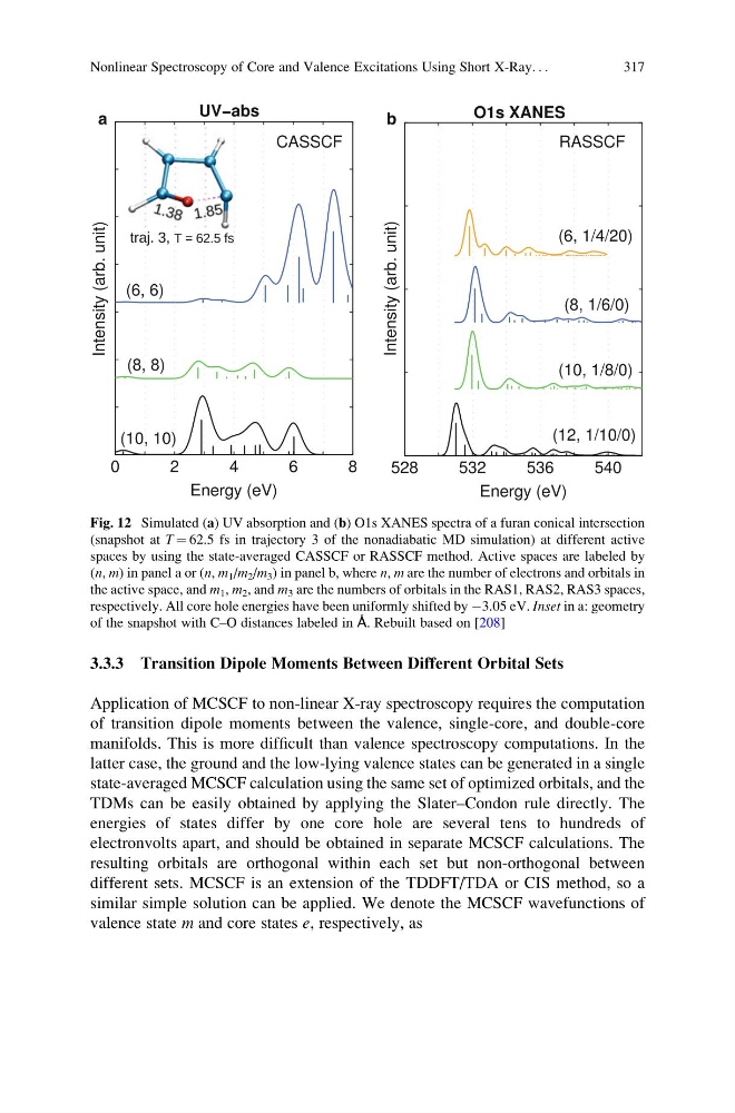
Fig. 12 Simulated (a) UV absorption and (b) O1s XANES spectra of a furan conical intersection
(snapshot at T ¼ 62.5 fs in trajectory 3 of the nonadiabatic MD simulation) at different active
spaces by using the state-averaged CASSCF or RASSCF method. Active spaces are labeled by
(n, m) in panel a or (n, m 1 /m 2 /m 3 ) in panel b, where n, m are the number of electrons and orbitals in
the active space, and m 1 , m 2 , and m 3 are the numbers of orbitals in the RAS1, RAS2, RAS3 spaces,
respectively. All core hole energies have been uniformly shifted by À3.05 eV. Inset in a: geometry
of the snapshot with C–O distances labeled in Å. Rebuilt based on [208]
Nonlinear Spectroscopy of Core and Valence Excitations Using Short X-Ray. . .
317
Application of MCSCF to non-linear X-ray spectroscopy requires the computation
of transition dipole moments between the valence, single-core, and double-core
manifolds. This is more difficult than valence spectroscopy computations. In the
latter case, the ground and the low-lying valence states can be generated in a single
state-averaged MCSCF calculation using the same set of optimized orbitals, and the
TDMs can be easily obtained by applying the Slater–Condon rule directly. The
energies of states differ by one core hole are several tens to hundreds of
electronvolts apart, and should be obtained in separate MCSCF calculations. The
resulting orbitals are orthogonal within each set but non-orthogonal between
different sets. MCSCF is an extension of the TDDFT/TDA or CIS method, so a
similar simple solution can be applied. We denote the MCSCF wavefunctions of
valence state m and core states e, respectively, as
b
a
Fig. 12 Simulated (a) UV absorption and (b) O1s XANES spectra of a furan conical intersection
(snapshot at T ¼ 62.5 fs in trajectory 3 of the nonadiabatic MD simulation) at different active
spaces by using the state-averaged CASSCF or RASSCF method. Active spaces are labeled by
(n, m) in panel a or (n, m 1 /m 2 /m 3 ) in panel b, where n, m are the number of electrons and orbitals in
the active space, and m 1 , m 2 , and m 3 are the numbers of orbitals in the RAS1, RAS2, RAS3 spaces,
respectively. All core hole energies have been uniformly shifted by À3.05 eV. Inset in a: geometry
of the snapshot with C–O distances labeled in Å. Rebuilt based on [208]
Nonlinear Spectroscopy of Core and Valence Excitations Using Short X-Ray. . .
317