

μ i t
ð Þ ¼ μ
0
i þ
X
ω
α i j Àω; ω
ð
ÞE
ω
j e
Àiωt
þ
1
2
X
ω 1 , ω 2
β i jk Àω s ; ω 1 , ω 2
ð
Þ E
ω 1
j E
ω 2
k e
Àiω s t
þ
1
6
X
ω 1 , ω 2 , ω 3
γ ijkl Àω s ; ω 1 , ω 2 , ω 3
ð
Þ E
ω 1
j E
ω 2
k E
ω 3
l e
Àiω s t
þ Á Á Á;
ð74Þ
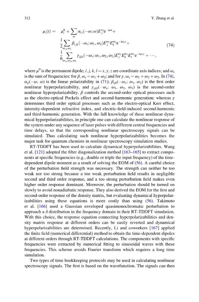
where μ
0 is the permanent dipole; i, j, k, l ¼ x, y, z are coordinate axis indices; and ω s
is the sum of frequencies: for β, ω s ¼ ω 1 þ ω 2 ; and for γ, ω s ¼ ω 1 þ ω 2 þ ω 3 . In (74),
α ij (Àω; ω) is the linear polarizability in (71); β ijk (Àω s ; ω 1 , ω 2 ) is the first order
nonlinear hyperpolarizability, and γ ijkl (Àω s ; ω 1 , ω 2 , ω 3 ) is the second-order
nonlinear hyperpolarizability. β controls the second-order optical processes such
as the electro-optical Pockels effect and second-harmonic generation; whereas γ
determines third order optical processes such as the electro-optical Kerr effect,
intensity-dependent refractive index, and electric-field-induced second-harmonic
and third-harmonic generation. With the full knowledge of these nonlinear dynamical hyperpolarizabilities, in principle one can calculate the nonlinear response of
the system under any sequence of laser pulses with different central frequencies and
time delays, so that the corresponding nonlinear spectroscopy signals can be
simulated. Thus calculating such nonlinear hyperpolarizabilities becomes the
major task for quantum chemists in nonlinear spectroscopy simulation studies.
RT-TDDFT has been used to calculate dynamical hyperpolarizabilities. Wang
et al. [121] adopted the filter diagonalization method [163–165] to extract components at specific frequencies (e.g., double or triple the input frequency) of the timedependent dipole moment as a result of solving the EOM of (56). A careful choice
of the perturbation field strength was necessary. The strength can neither be too
weak nor too strong because a too weak perturbation field results in negligible
second and third order response, and a too strong perturbation field makes even
higher order response dominant. Moreover, the perturbation should be turned on
slowly to avoid nonadiabatic response. They also derived the EOM for the first and
second-order response of the density matrix, but evaluating dynamical hyperpolarizabilities using these equations is more costly than using (56). Takimoto
et al. [166] used a Gaussian enveloped quasimonochromatic perturbation to
approach a δ distribution in the frequency domain in their RT-TDDFT simulation.
With this choice, the response equation connecting hyperpolarizabilities and density matrix response at different orders can be easily reverted and dynamical
hyperpolarizabilities are determined. Recently, Li and coworkers [167] applied
the finite field (numerical differential) method to obtain the time-dependent dipoles
at different orders through RT-TDDFT calculations. The components with specific
frequencies were extracted by numerical fitting to sinusoidal waves with these
frequencies. This scheme avoids Fourier transform which requires a long time
simulation.
Two types of time bookkeeping protocols may be used in calculating nonlinear
spectroscopy signals. The first is based on the wavefunction. The signals can then
312
Y. Zhang et al.
ð Þ ¼ μ
0
i þ
X
ω
α i j Àω; ω
ð
ÞE
ω
j e
Àiωt
þ
1
2
X
ω 1 , ω 2
β i jk Àω s ; ω 1 , ω 2
ð
Þ E
ω 1
j E
ω 2
k e
Àiω s t
þ
1
6
X
ω 1 , ω 2 , ω 3
γ ijkl Àω s ; ω 1 , ω 2 , ω 3
ð
Þ E
ω 1
j E
ω 2
k E
ω 3
l e
Àiω s t
þ Á Á Á;
ð74Þ
where μ
0 is the permanent dipole; i, j, k, l ¼ x, y, z are coordinate axis indices; and ω s
is the sum of frequencies: for β, ω s ¼ ω 1 þ ω 2 ; and for γ, ω s ¼ ω 1 þ ω 2 þ ω 3 . In (74),
α ij (Àω; ω) is the linear polarizability in (71); β ijk (Àω s ; ω 1 , ω 2 ) is the first order
nonlinear hyperpolarizability, and γ ijkl (Àω s ; ω 1 , ω 2 , ω 3 ) is the second-order
nonlinear hyperpolarizability. β controls the second-order optical processes such
as the electro-optical Pockels effect and second-harmonic generation; whereas γ
determines third order optical processes such as the electro-optical Kerr effect,
intensity-dependent refractive index, and electric-field-induced second-harmonic
and third-harmonic generation. With the full knowledge of these nonlinear dynamical hyperpolarizabilities, in principle one can calculate the nonlinear response of
the system under any sequence of laser pulses with different central frequencies and
time delays, so that the corresponding nonlinear spectroscopy signals can be
simulated. Thus calculating such nonlinear hyperpolarizabilities becomes the
major task for quantum chemists in nonlinear spectroscopy simulation studies.
RT-TDDFT has been used to calculate dynamical hyperpolarizabilities. Wang
et al. [121] adopted the filter diagonalization method [163–165] to extract components at specific frequencies (e.g., double or triple the input frequency) of the timedependent dipole moment as a result of solving the EOM of (56). A careful choice
of the perturbation field strength was necessary. The strength can neither be too
weak nor too strong because a too weak perturbation field results in negligible
second and third order response, and a too strong perturbation field makes even
higher order response dominant. Moreover, the perturbation should be turned on
slowly to avoid nonadiabatic response. They also derived the EOM for the first and
second-order response of the density matrix, but evaluating dynamical hyperpolarizabilities using these equations is more costly than using (56). Takimoto
et al. [166] used a Gaussian enveloped quasimonochromatic perturbation to
approach a δ distribution in the frequency domain in their RT-TDDFT simulation.
With this choice, the response equation connecting hyperpolarizabilities and density matrix response at different orders can be easily reverted and dynamical
hyperpolarizabilities are determined. Recently, Li and coworkers [167] applied
the finite field (numerical differential) method to obtain the time-dependent dipoles
at different orders through RT-TDDFT calculations. The components with specific
frequencies were extracted by numerical fitting to sinusoidal waves with these
frequencies. This scheme avoids Fourier transform which requires a long time
simulation.
Two types of time bookkeeping protocols may be used in calculating nonlinear
spectroscopy signals. The first is based on the wavefunction. The signals can then
312
Y. Zhang et al.