

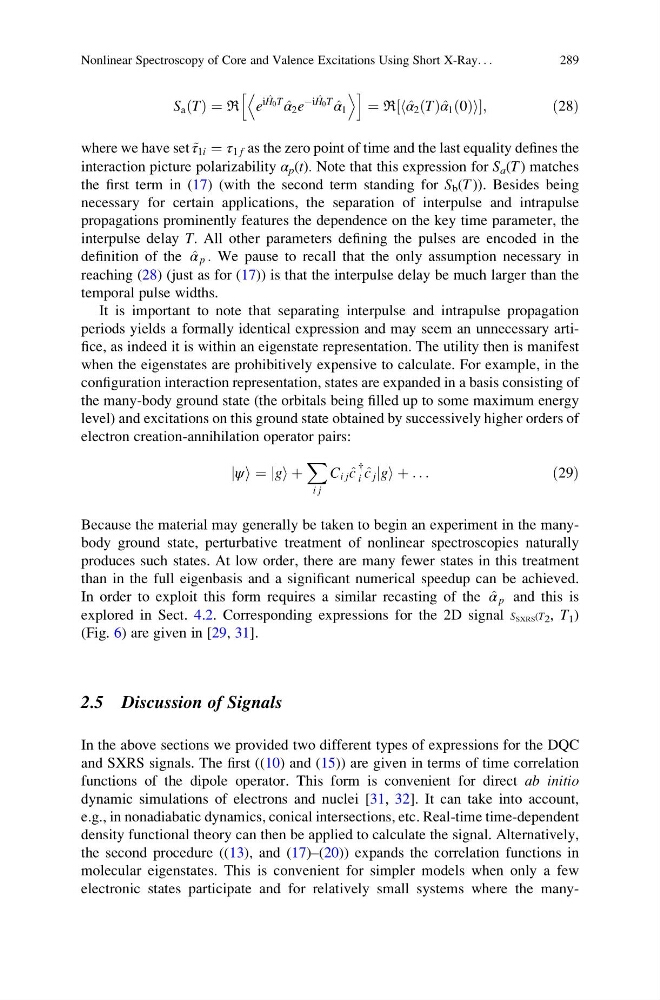
S a T
ð Þ ¼ ℜ e
i ^
H 0 T
^
α 2 e
Ài ^
H 0 T
^
α 1
D
E
h
i
¼ ℜ ^
α 2 T
ð Þ^ α 1 0
ð Þ
h
i
½
;
ð28Þ
where we have set ~
τ 1i ¼ τ 1 f as the zero point of time and the last equality defines the
interaction picture polarizability α p (t). Note that this expression for S a (T ) matches
the first term in (17) (with the second term standing for S b (T )). Besides being
necessary for certain applications, the separation of interpulse and intrapulse
propagations prominently features the dependence on the key time parameter, the
interpulse delay T. All other parameters defining the pulses are encoded in the
definition of the ^
α p . We pause to recall that the only assumption necessary in
reaching (28) (just as for (17)) is that the interpulse delay be much larger than the
temporal pulse widths.
It is important to note that separating interpulse and intrapulse propagation
periods yields a formally identical expression and may seem an unnecessary artifice, as indeed it is within an eigenstate representation. The utility then is manifest
when the eigenstates are prohibitively expensive to calculate. For example, in the
configuration interaction representation, states are expanded in a basis consisting of
the many-body ground state (the orbitals being filled up to some maximum energy
level) and excitations on this ground state obtained by successively higher orders of
electron creation-annihilation operator pairs:
ψ
j i ¼ g
j i þ
X
i j
C i j ^
c
{
i ^
c j g
j i þ . . .
ð29Þ
Because the material may generally be taken to begin an experiment in the manybody ground state, perturbative treatment of nonlinear spectroscopies naturally
produces such states. At low order, there are many fewer states in this treatment
than in the full eigenbasis and a significant numerical speedup can be achieved.
In order to exploit this form requires a similar recasting of the ^
α p and this is
explored in Sect. 4.2. Corresponding expressions for the 2D signal S SXRS (T 2 , T 1 )
(Fig. 6) are given in [29, 31].
2.5 Discussion of Signals
In the above sections we provided two different types of expressions for the DQC
and SXRS signals. The first ((10) and (15)) are given in terms of time correlation
functions of the dipole operator. This form is convenient for direct ab initio
dynamic simulations of electrons and nuclei [31, 32]. It can take into account,
e.g., in nonadiabatic dynamics, conical intersections, etc. Real-time time-dependent
density functional theory can then be applied to calculate the signal. Alternatively,
the second procedure ((13), and (17)–(20)) expands the correlation functions in
molecular eigenstates. This is convenient for simpler models when only a few
electronic states participate and for relatively small systems where the manyNonlinear Spectroscopy of Core and Valence Excitations Using Short X-Ray. . .
289
ð Þ ¼ ℜ e
i ^
H 0 T
^
α 2 e
Ài ^
H 0 T
^
α 1
D
E
h
i
¼ ℜ ^
α 2 T
ð Þ^ α 1 0
ð Þ
h
i
½
;
ð28Þ
where we have set ~
τ 1i ¼ τ 1 f as the zero point of time and the last equality defines the
interaction picture polarizability α p (t). Note that this expression for S a (T ) matches
the first term in (17) (with the second term standing for S b (T )). Besides being
necessary for certain applications, the separation of interpulse and intrapulse
propagations prominently features the dependence on the key time parameter, the
interpulse delay T. All other parameters defining the pulses are encoded in the
definition of the ^
α p . We pause to recall that the only assumption necessary in
reaching (28) (just as for (17)) is that the interpulse delay be much larger than the
temporal pulse widths.
It is important to note that separating interpulse and intrapulse propagation
periods yields a formally identical expression and may seem an unnecessary artifice, as indeed it is within an eigenstate representation. The utility then is manifest
when the eigenstates are prohibitively expensive to calculate. For example, in the
configuration interaction representation, states are expanded in a basis consisting of
the many-body ground state (the orbitals being filled up to some maximum energy
level) and excitations on this ground state obtained by successively higher orders of
electron creation-annihilation operator pairs:
ψ
j i ¼ g
j i þ
X
i j
C i j ^
c
{
i ^
c j g
j i þ . . .
ð29Þ
Because the material may generally be taken to begin an experiment in the manybody ground state, perturbative treatment of nonlinear spectroscopies naturally
produces such states. At low order, there are many fewer states in this treatment
than in the full eigenbasis and a significant numerical speedup can be achieved.
In order to exploit this form requires a similar recasting of the ^
α p and this is
explored in Sect. 4.2. Corresponding expressions for the 2D signal S SXRS (T 2 , T 1 )
(Fig. 6) are given in [29, 31].
2.5 Discussion of Signals
In the above sections we provided two different types of expressions for the DQC
and SXRS signals. The first ((10) and (15)) are given in terms of time correlation
functions of the dipole operator. This form is convenient for direct ab initio
dynamic simulations of electrons and nuclei [31, 32]. It can take into account,
e.g., in nonadiabatic dynamics, conical intersections, etc. Real-time time-dependent
density functional theory can then be applied to calculate the signal. Alternatively,
the second procedure ((13), and (17)–(20)) expands the correlation functions in
molecular eigenstates. This is convenient for simpler models when only a few
electronic states participate and for relatively small systems where the manyNonlinear Spectroscopy of Core and Valence Excitations Using Short X-Ray. . .
289