

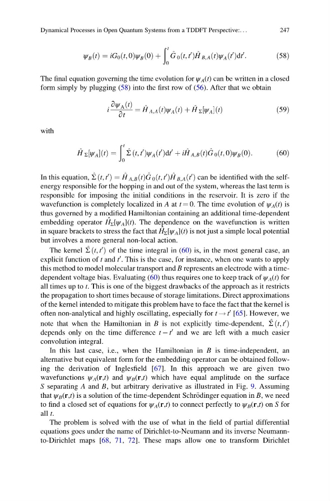
ψ B t
ð Þ ¼ iG 0 t; 0
ð Þψ B 0
ð Þ þ
ð t
0
^
G 0 t, t
0
ð Þ ^
H B, A t
ð Þψ A t
0
ð Þdt
0
:
ð58Þ
The final equation governing the time evolution for ψ A (t) can be written in a closed
form simply by plugging (58) into the first row of (56). After that we obtain
i
∂ψ Α t
ð Þ
∂t
¼ ^
H A, A t
ð Þψ A t
ð Þ þ ^
H Σ ψ A
½ t
ð Þ
ð59Þ
with
^
H Σ ψ A
½ t
ð Þ ¼
ð t
0
^
Σ t, t
0
ð Þψ A t
0
ð Þdt
0
þ i ^
H A, B t
ð Þ ^
G 0 t; 0
ð Þψ B 0
ð Þ:
ð60Þ
In this equation, ^
Σ t, t
0
ð Þ ¼ ^
H A, B t
ð Þ ^
G 0 t, t
0
ð Þ ^
H B, A t
0
ð Þ can be identified with the selfenergy responsible for the hopping in and out of the system, whereas the last term is
responsible for imposing the initial conditions in the reservoir. It is zero if the
wavefunction is completely localized in A at t ¼ 0. The time evolution of ψ A (t) is
thus governed by a modified Hamiltonian containing an additional time-dependent
embedding operator H ˆ Σ [ψ A ](t). The dependence on the wavefunction is written
in square brackets to stress the fact that H ˆ Σ [ψ A ](t) is not just a simple local potential
but involves a more general non-local action.
The kernel ^
Σ t, t
0
ð Þ of the time integral in (60) is, in the most general case, an
explicit function of t and t
0 . This is the case, for instance, when one wants to apply
this method to model molecular transport and B represents an electrode with a timedependent voltage bias. Evaluating (60) thus requires one to keep track of ψ A (t) for
all times up to t. This is one of the biggest drawbacks of the approach as it restricts
the propagation to short times because of storage limitations. Direct approximations
of the kernel intended to mitigate this problem have to face the fact that the kernel is
often non-analytical and highly oscillating, especially for t ! t
0 [65]. However, we
note that when the Hamiltonian in B is not explicitly time-dependent, ^
Σ t; t
0
ð Þ
depends only on the time difference t À t
0 and we are left with a much easier
convolution integral.
In this last case, i.e., when the Hamiltonian in B is time-independent, an
alternative but equivalent form for the embedding operator can be obtained following the derivation of Inglesfield [67]. In this approach we are given two
wavefunctions ψ A (r,t) and ψ B (r,t) which have equal amplitude on the surface
S separating A and B, but arbitrary derivative as illustrated in Fig. 9. Assuming
that ψ B (r,t) is a solution of the time-dependent Schr€ odinger equation in B, we need
to find a closed set of equations for ψ A (r,t) to connect perfectly to ψ B (r,t) on S for
all t.
The problem is solved with the use of what in the field of partial differential
equations goes under the name of Dirichlet-to-Neumann and its inverse Neumannto-Dirichlet maps [68, 71, 72]. These maps allow one to transform Dirichlet
Dynamical Processes in Open Quantum Systems from a TDDFT Perspective:. . .
247
ð Þ ¼ iG 0 t; 0
ð Þψ B 0
ð Þ þ
ð t
0
^
G 0 t, t
0
ð Þ ^
H B, A t
ð Þψ A t
0
ð Þdt
0
:
ð58Þ
The final equation governing the time evolution for ψ A (t) can be written in a closed
form simply by plugging (58) into the first row of (56). After that we obtain
i
∂ψ Α t
ð Þ
∂t
¼ ^
H A, A t
ð Þψ A t
ð Þ þ ^
H Σ ψ A
½ t
ð Þ
ð59Þ
with
^
H Σ ψ A
½ t
ð Þ ¼
ð t
0
^
Σ t, t
0
ð Þψ A t
0
ð Þdt
0
þ i ^
H A, B t
ð Þ ^
G 0 t; 0
ð Þψ B 0
ð Þ:
ð60Þ
In this equation, ^
Σ t, t
0
ð Þ ¼ ^
H A, B t
ð Þ ^
G 0 t, t
0
ð Þ ^
H B, A t
0
ð Þ can be identified with the selfenergy responsible for the hopping in and out of the system, whereas the last term is
responsible for imposing the initial conditions in the reservoir. It is zero if the
wavefunction is completely localized in A at t ¼ 0. The time evolution of ψ A (t) is
thus governed by a modified Hamiltonian containing an additional time-dependent
embedding operator H ˆ Σ [ψ A ](t). The dependence on the wavefunction is written
in square brackets to stress the fact that H ˆ Σ [ψ A ](t) is not just a simple local potential
but involves a more general non-local action.
The kernel ^
Σ t, t
0
ð Þ of the time integral in (60) is, in the most general case, an
explicit function of t and t
0 . This is the case, for instance, when one wants to apply
this method to model molecular transport and B represents an electrode with a timedependent voltage bias. Evaluating (60) thus requires one to keep track of ψ A (t) for
all times up to t. This is one of the biggest drawbacks of the approach as it restricts
the propagation to short times because of storage limitations. Direct approximations
of the kernel intended to mitigate this problem have to face the fact that the kernel is
often non-analytical and highly oscillating, especially for t ! t
0 [65]. However, we
note that when the Hamiltonian in B is not explicitly time-dependent, ^
Σ t; t
0
ð Þ
depends only on the time difference t À t
0 and we are left with a much easier
convolution integral.
In this last case, i.e., when the Hamiltonian in B is time-independent, an
alternative but equivalent form for the embedding operator can be obtained following the derivation of Inglesfield [67]. In this approach we are given two
wavefunctions ψ A (r,t) and ψ B (r,t) which have equal amplitude on the surface
S separating A and B, but arbitrary derivative as illustrated in Fig. 9. Assuming
that ψ B (r,t) is a solution of the time-dependent Schr€ odinger equation in B, we need
to find a closed set of equations for ψ A (r,t) to connect perfectly to ψ B (r,t) on S for
all t.
The problem is solved with the use of what in the field of partial differential
equations goes under the name of Dirichlet-to-Neumann and its inverse Neumannto-Dirichlet maps [68, 71, 72]. These maps allow one to transform Dirichlet
Dynamical Processes in Open Quantum Systems from a TDDFT Perspective:. . .
247