

ϕ θ rt
ð Þ ¼ e
Ài ^
H θ t
ϕ
0
θ r
ð Þ ¼ e
Àiε θ t
ϕ
0
θ r
ð Þ:
ð55Þ
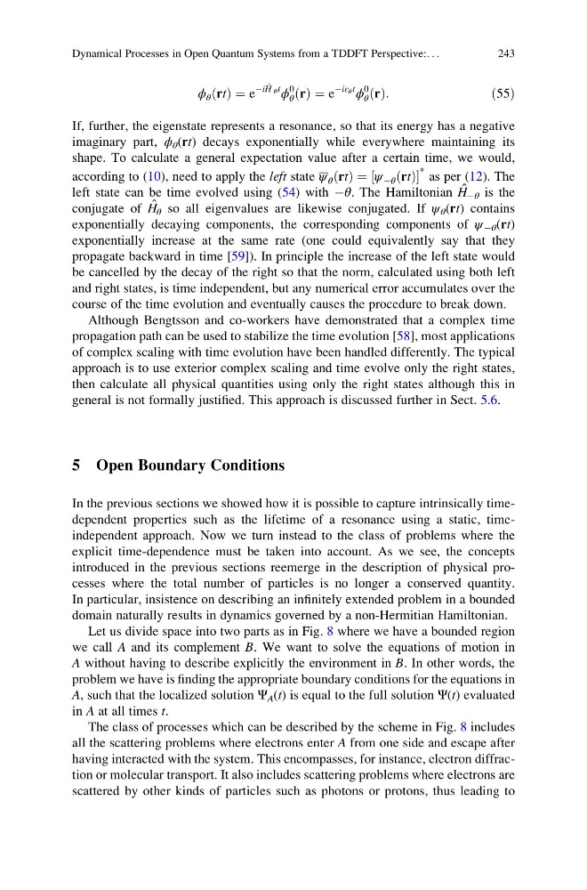
If, further, the eigenstate represents a resonance, so that its energy has a negative
imaginary part, ϕ θ (rt) decays exponentially while everywhere maintaining its
shape. To calculate a general expectation value after a certain time, we would,
according to (10), need to apply the left state ψ θ rt
ð Þ ¼ ψ Àθ rt
ð Þ
½
* as per (12). The
left state can be time evolved using (54) with Àθ. The Hamiltonian H ˆ Àθ is the
conjugate of H ˆ θ so all eigenvalues are likewise conjugated. If ψ θ (rt) contains
exponentially decaying components, the corresponding components of ψ Àθ (rt)
exponentially increase at the same rate (one could equivalently say that they
propagate backward in time [59]). In principle the increase of the left state would
be cancelled by the decay of the right so that the norm, calculated using both left
and right states, is time independent, but any numerical error accumulates over the
course of the time evolution and eventually causes the procedure to break down.
Although Bengtsson and co-workers have demonstrated that a complex time
propagation path can be used to stabilize the time evolution [58], most applications
of complex scaling with time evolution have been handled differently. The typical
approach is to use exterior complex scaling and time evolve only the right states,
then calculate all physical quantities using only the right states although this in
general is not formally justified. This approach is discussed further in Sect. 5.6.
5 Open Boundary Conditions
In the previous sections we showed how it is possible to capture intrinsically timedependent properties such as the lifetime of a resonance using a static, timeindependent approach. Now we turn instead to the class of problems where the
explicit time-dependence must be taken into account. As we see, the concepts
introduced in the previous sections reemerge in the description of physical processes where the total number of particles is no longer a conserved quantity.
In particular, insistence on describing an infinitely extended problem in a bounded
domain naturally results in dynamics governed by a non-Hermitian Hamiltonian.
Let us divide space into two parts as in Fig. 8 where we have a bounded region
we call A and its complement B. We want to solve the equations of motion in
A without having to describe explicitly the environment in B. In other words, the
problem we have is finding the appropriate boundary conditions for the equations in
A, such that the localized solution Ψ A (t) is equal to the full solution Ψ(t) evaluated
in A at all times t.
The class of processes which can be described by the scheme in Fig. 8 includes
all the scattering problems where electrons enter A from one side and escape after
having interacted with the system. This encompasses, for instance, electron diffraction or molecular transport. It also includes scattering problems where electrons are
scattered by other kinds of particles such as photons or protons, thus leading to
Dynamical Processes in Open Quantum Systems from a TDDFT Perspective:. . .
243
ð Þ ¼ e
Ài ^
H θ t
ϕ
0
θ r
ð Þ ¼ e
Àiε θ t
ϕ
0
θ r
ð Þ:
ð55Þ
If, further, the eigenstate represents a resonance, so that its energy has a negative
imaginary part, ϕ θ (rt) decays exponentially while everywhere maintaining its
shape. To calculate a general expectation value after a certain time, we would,
according to (10), need to apply the left state ψ θ rt
ð Þ ¼ ψ Àθ rt
ð Þ
½
* as per (12). The
left state can be time evolved using (54) with Àθ. The Hamiltonian H ˆ Àθ is the
conjugate of H ˆ θ so all eigenvalues are likewise conjugated. If ψ θ (rt) contains
exponentially decaying components, the corresponding components of ψ Àθ (rt)
exponentially increase at the same rate (one could equivalently say that they
propagate backward in time [59]). In principle the increase of the left state would
be cancelled by the decay of the right so that the norm, calculated using both left
and right states, is time independent, but any numerical error accumulates over the
course of the time evolution and eventually causes the procedure to break down.
Although Bengtsson and co-workers have demonstrated that a complex time
propagation path can be used to stabilize the time evolution [58], most applications
of complex scaling with time evolution have been handled differently. The typical
approach is to use exterior complex scaling and time evolve only the right states,
then calculate all physical quantities using only the right states although this in
general is not formally justified. This approach is discussed further in Sect. 5.6.
5 Open Boundary Conditions
In the previous sections we showed how it is possible to capture intrinsically timedependent properties such as the lifetime of a resonance using a static, timeindependent approach. Now we turn instead to the class of problems where the
explicit time-dependence must be taken into account. As we see, the concepts
introduced in the previous sections reemerge in the description of physical processes where the total number of particles is no longer a conserved quantity.
In particular, insistence on describing an infinitely extended problem in a bounded
domain naturally results in dynamics governed by a non-Hermitian Hamiltonian.
Let us divide space into two parts as in Fig. 8 where we have a bounded region
we call A and its complement B. We want to solve the equations of motion in
A without having to describe explicitly the environment in B. In other words, the
problem we have is finding the appropriate boundary conditions for the equations in
A, such that the localized solution Ψ A (t) is equal to the full solution Ψ(t) evaluated
in A at all times t.
The class of processes which can be described by the scheme in Fig. 8 includes
all the scattering problems where electrons enter A from one side and escape after
having interacted with the system. This encompasses, for instance, electron diffraction or molecular transport. It also includes scattering problems where electrons are
scattered by other kinds of particles such as photons or protons, thus leading to
Dynamical Processes in Open Quantum Systems from a TDDFT Perspective:. . .
243