

V x
ð Þ ¼
0, 0 x < a,
V 0 , a x < b,
0,
b x;
8
<
:
ð26Þ
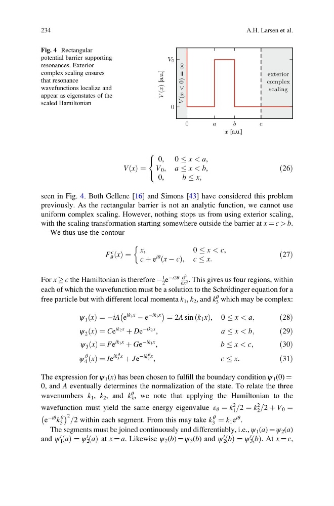
seen in Fig. 4. Both Gellene [16] and Simons [43] have considered this problem
previously. As the rectangular barrier is not an analytic function, we cannot use
uniform complex scaling. However, nothing stops us from using exterior scaling,
with the scaling transformation starting somewhere outside the barrier at x ¼ c > b.
We thus use the contour
F
c
θ x
ð Þ ¼
x,
0 x < c,
c þ e
iθ x À c
ð
Þ, c x:
&
ð27Þ
For x ! c the Hamiltonian is therefore À
1
2 e
Ài2θ d
2
dx 2 . This gives us four regions, within
each of which the wavefunction must be a solution to the Schr€ odinger equation for a
free particle but with different local momenta k 1 , k 2 , and k
θ
3 which may be complex:
ψ 1 x
ð Þ ¼ ÀiA e
ik 1 x
À e
Àik 1 x
À
Á ¼ 2A sin k 1 x
ð Þ, 0 x < a;
ð28Þ
ψ 2 x
ð Þ ¼ Ce
ik 2 x
þ De
Àik 2 x ,
a x < b;
ð29Þ
ψ 3 x
ð Þ ¼ Fe
ik 1 x
þ Ge
Àik 1 x ,
b x < c;
ð30Þ
ψ
θ
4 x
ð Þ ¼ Ie
ik
θ
3 x
þ Je
Àik
θ
3 x ,
c x:
ð31Þ
The expression for ψ 1 (x) has been chosen to fulfill the boundary condition ψ 1 (0) ¼
0, and A eventually determines the normalization of the state. To relate the three
wavenumbers k 1 , k 2 , and k
θ
3 , we note that applying the Hamiltonian to the
wavefunction must yield the same energy eigenvalue ε θ ¼ k
2
1 =2 ¼ k
2
2 =2 þ V 0 ¼
e
Àiθ k
θ
3
À
Á 2 =2 within each segment. From this may take k
θ
3 ¼ k 1 e
iθ .
The segments must be joined continuously and differentiably, i.e., ψ 1 (a) ¼ ψ 2 (a)
and ψ 1
0 a
ð Þ ¼ ψ 2
0 a
ð Þ at x ¼ a. Likewise ψ 2 (b) ¼ ψ 3 (b) and ψ 2
0 b
ð Þ ¼ ψ 3
0 b
ð Þ. At x ¼ c,
0
a
b
c
x [a.u.]
0
V 0
V (x)
[a.u.]
V (x
< 0) =
∞
exterior
complex
scaling
Fig. 4 Rectangular
potential barrier supporting
resonances. Exterior
complex scaling ensures
that resonance
wavefunctions localize and
appear as eigenstates of the
scaled Hamiltonian
234
A.H. Larsen et al.
ð Þ ¼
0, 0 x < a,
V 0 , a x < b,
0,
b x;
8
<
:
ð26Þ
seen in Fig. 4. Both Gellene [16] and Simons [43] have considered this problem
previously. As the rectangular barrier is not an analytic function, we cannot use
uniform complex scaling. However, nothing stops us from using exterior scaling,
with the scaling transformation starting somewhere outside the barrier at x ¼ c > b.
We thus use the contour
F
c
θ x
ð Þ ¼
x,
0 x < c,
c þ e
iθ x À c
ð
Þ, c x:
&
ð27Þ
For x ! c the Hamiltonian is therefore À
1
2 e
Ài2θ d
2
dx 2 . This gives us four regions, within
each of which the wavefunction must be a solution to the Schr€ odinger equation for a
free particle but with different local momenta k 1 , k 2 , and k
θ
3 which may be complex:
ψ 1 x
ð Þ ¼ ÀiA e
ik 1 x
À e
Àik 1 x
À
Á ¼ 2A sin k 1 x
ð Þ, 0 x < a;
ð28Þ
ψ 2 x
ð Þ ¼ Ce
ik 2 x
þ De
Àik 2 x ,
a x < b;
ð29Þ
ψ 3 x
ð Þ ¼ Fe
ik 1 x
þ Ge
Àik 1 x ,
b x < c;
ð30Þ
ψ
θ
4 x
ð Þ ¼ Ie
ik
θ
3 x
þ Je
Àik
θ
3 x ,
c x:
ð31Þ
The expression for ψ 1 (x) has been chosen to fulfill the boundary condition ψ 1 (0) ¼
0, and A eventually determines the normalization of the state. To relate the three
wavenumbers k 1 , k 2 , and k
θ
3 , we note that applying the Hamiltonian to the
wavefunction must yield the same energy eigenvalue ε θ ¼ k
2
1 =2 ¼ k
2
2 =2 þ V 0 ¼
e
Àiθ k
θ
3
À
Á 2 =2 within each segment. From this may take k
θ
3 ¼ k 1 e
iθ .
The segments must be joined continuously and differentiably, i.e., ψ 1 (a) ¼ ψ 2 (a)
and ψ 1
0 a
ð Þ ¼ ψ 2
0 a
ð Þ at x ¼ a. Likewise ψ 2 (b) ¼ ψ 3 (b) and ψ 2
0 b
ð Þ ¼ ψ 3
0 b
ð Þ. At x ¼ c,
0
a
b
c
x [a.u.]
0
V 0
V (x)
[a.u.]
V (x
< 0) =
∞
exterior
complex
scaling
Fig. 4 Rectangular
potential barrier supporting
resonances. Exterior
complex scaling ensures
that resonance
wavefunctions localize and
appear as eigenstates of the
scaled Hamiltonian
234
A.H. Larsen et al.