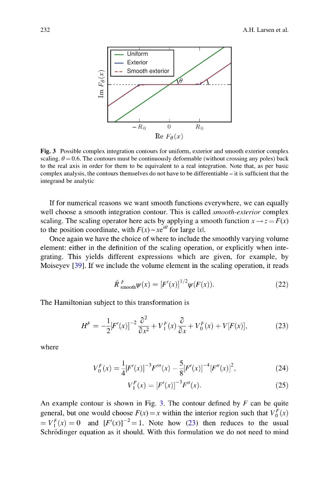
If for numerical reasons we want smooth functions everywhere, we can equally
well choose a smooth integration contour. This is called smooth-exterior complex
scaling. The scaling operator here acts by applying a smooth function x ! z ¼ F(x)
to the position coordinate, with F(x) ~ xe
iθ for large |x|.
Once again we have the choice of where to include the smoothly varying volume
element: either in the definition of the scaling operation, or explicitly when integrating. This yields different expressions which are given, for example, by
Moiseyev [39]. If we include the volume element in the scaling operation, it reads
^
R
F
smooth ψ x
ð Þ ¼ F
0 x
ð Þ
½
Š
1=2 ψ F x
ð Þ
ð
Þ:
ð22Þ
The Hamiltonian subject to this transformation is
H
F
¼ À
1
2
F
0 x
ð Þ
½
Š
À2 ∂
2
∂x 2 þ V
F
1 x
ð Þ
∂
∂x
þ V
F
0 x
ð Þ þ V F x
ð Þ
½
Š;
ð23Þ
where
V
F
0 x
ð Þ ¼
1
4
F
0 x
ð Þ
½
Š
À3 F
000 x
ð Þ À
5
8
F
0 x
ð Þ
½
Š
À4 F
00 x
ð Þ
½
Š
2 ;
ð24Þ
V
F
1 x
ð Þ ¼ F
0 x
ð Þ
½
Š
À3 F
00 x
ð Þ:
ð25Þ
An example contour is shown in Fig. 3. The contour defined by F can be quite
general, but one would choose F(x) ¼ x within the interior region such that V
F
0 x
ð Þ
¼ V
F
1 x
ð Þ ¼ 0 and [F
0 (x)]
À2
¼ 1. Note how (23) then reduces to the usual
Schr€ odinger equation as it should. With this formulation we do not need to mind
− R 0
0
R 0
Re F θ (x)
Im F
θ (x)
θ
Uniform
Exterior
Smooth exterior
Fig. 3 Possible complex integration contours for uniform, exterior and smooth exterior complex
scaling. θ ¼ 0.6. The contours must be continuously deformable (without crossing any poles) back
to the real axis in order for them to be equivalent to a real integration. Note that, as per basic
complex analysis, the contours themselves do not have to be differentiable – it is sufficient that the
integrand be analytic
232
A.H. Larsen et al.