

K
BSE
iak, jbk 0 ¼ K
H
iak, jbk 0 þ K
W
iak, jbk 0 ;
ð69Þ
where
K
W
iak, jbk 0 ¼ À
1
V
X
GG 0
W GG 0 q
ð Þ ik
h je
i qþG
ð
Þ Ár jk
j i bk
0
h je
Ài qþG
0
ð
Þ Á r ak
0
j i:
ð70Þ
The Hartree part is the same as in TDDFT, but the xc part is replaced by a coupling
matrix featuring the screened interaction (62). In practice, one ignores the frequency dependence of W; explicitly, one finds
W GG 0 q, ω ¼ 0
ð
Þ¼
4πε
À1
GG 0 q, ω ¼ 0
ð
Þ
q þ G 0
j
j
2
:
ð71Þ
Let us now compare the two coupling matrices K
xc and K
W . Two main differences
become apparent: first, the order of the band indices i, j, a, b is different; second, the
xc matrix only depends on the long-range (q ¼ 0) behavior, while the W matrix also
depends on other values of q.
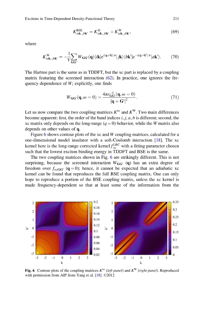
Figure 6 shows contour plots of the xc and W coupling matrices, calculated for a
one-dimensional model insulator with a soft-Coulomb interaction [18]. The xc
kernel here is the long-range corrected kernel f
LRC
xc with a fitting parameter chosen
such that the lowest exciton binding energy in TDDFT and BSE is the same.
The two coupling matrices shown in Fig. 6 are strikingly different. This is not
surprising, because the screened interaction W GG
0 (q) has an extra degree of
freedom over f xcGG
0 (q ¼ 0); hence, it cannot be expected that an adiabatic xc
kernel can be found that reproduces the full BSE coupling matrix. One can only
hope to reproduce a portion of the BSE coupling matrix, unless the xc kernel is
made frequency-dependent so that at least some of the information from the
Fig. 6 Contour plots of the coupling matrices K
xc (left panel) and K
W (right panel). Reproduced
with permission from AIP from Yang et al. [18]. ©2012
Excitons in Time-Dependent Density-Functional Theory
211
BSE
iak, jbk 0 ¼ K
H
iak, jbk 0 þ K
W
iak, jbk 0 ;
ð69Þ
where
K
W
iak, jbk 0 ¼ À
1
V
X
GG 0
W GG 0 q
ð Þ ik
h je
i qþG
ð
Þ Ár jk
j i bk
0
h je
Ài qþG
0
ð
Þ Á r ak
0
j i:
ð70Þ
The Hartree part is the same as in TDDFT, but the xc part is replaced by a coupling
matrix featuring the screened interaction (62). In practice, one ignores the frequency dependence of W; explicitly, one finds
W GG 0 q, ω ¼ 0
ð
Þ¼
4πε
À1
GG 0 q, ω ¼ 0
ð
Þ
q þ G 0
j
j
2
:
ð71Þ
Let us now compare the two coupling matrices K
xc and K
W . Two main differences
become apparent: first, the order of the band indices i, j, a, b is different; second, the
xc matrix only depends on the long-range (q ¼ 0) behavior, while the W matrix also
depends on other values of q.
Figure 6 shows contour plots of the xc and W coupling matrices, calculated for a
one-dimensional model insulator with a soft-Coulomb interaction [18]. The xc
kernel here is the long-range corrected kernel f
LRC
xc with a fitting parameter chosen
such that the lowest exciton binding energy in TDDFT and BSE is the same.
The two coupling matrices shown in Fig. 6 are strikingly different. This is not
surprising, because the screened interaction W GG
0 (q) has an extra degree of
freedom over f xcGG
0 (q ¼ 0); hence, it cannot be expected that an adiabatic xc
kernel can be found that reproduces the full BSE coupling matrix. One can only
hope to reproduce a portion of the BSE coupling matrix, unless the xc kernel is
made frequency-dependent so that at least some of the information from the
Fig. 6 Contour plots of the coupling matrices K
xc (left panel) and K
W (right panel). Reproduced
with permission from AIP from Yang et al. [18]. ©2012
Excitons in Time-Dependent Density-Functional Theory
211