case, the former was selected. It should be emphasized that optimization can only
be achieved for the environment reflected in the model. Great care was taken
therefore to reflect all the meaningful, worthwhile options known to be available.
There are many refinery variables that are of a nonlinear nature. Among these
nonlinearities are the effects of blending on motor gasoline, the capital expenditures
in relation to size of the units, and many severity effects within the various
processes. When these effects could be described on a cost basis by a CONVEX
curve, they were generally included in the model as linear segments of a curve (see
Fig. 18).
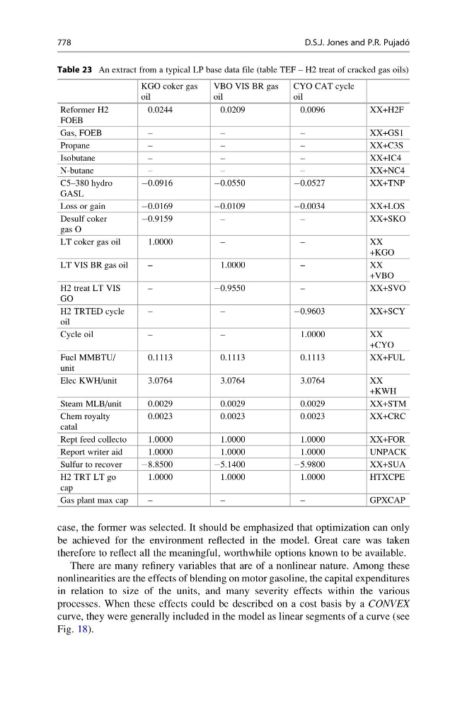
Table 23 An extract from a typical LP base data file (table TEF – H2 treat of cracked gas oils)
KGO coker gas
oil
VBO VIS BR gas
oil
CYO CAT cycle
oil
Reformer H2
FOEB
0.0244
0.0209
0.0096
XX+H2F
Gas, FOEB
–
–
–
XX+GS1
Propane
–
–
–
XX+C3S
Isobutane
–
–
–
XX+IC4
N-butane
–
–
–
XX+NC4
C5–380 hydro
GASL
À0.0916
À0.0550
À0.0527
XX+TNP
Loss or gain
À0.0169
À0.0109
À0.0034
XX+LOS
Desulf coker
gas O
À0.9159
–
–
XX+SKO
LT coker gas oil
1.0000
–
–
XX
+KGO
LT VIS BR gas oil
–
1.0000
–
XX
+VBO
H2 treat LT VIS
GO
–
À0.9550
–
XX+SVO
H2 TRTED cycle
oil
–
–
À0.9603
XX+SCY
Cycle oil
–
–
1.0000
XX
+CYO
Fuel MMBTU/
unit
0.1113
0.1113
0.1113
XX+FUL
Elec KWH/unit
3.0764
3.0764
3.0764
XX
+KWH
Steam MLB/unit
0.0029
0.0029
0.0029
XX+STM
Chem royalty
catal
0.0023
0.0023
0.0023
XX+CRC
Rept feed collecto
1.0000
1.0000
1.0000
XX+FOR
Report writer aid
1.0000
1.0000
1.0000
UNPACK
Sulfur to recover
À8.8500
À5.1400
À5.9800
XX+SUA
H2 TRT LT go
cap
1.0000
1.0000
1.0000
HTXCPE
Gas plant max cap
–
–
–
GPXCAP
778
D.S.J. Jones and P.R. Pujado ´