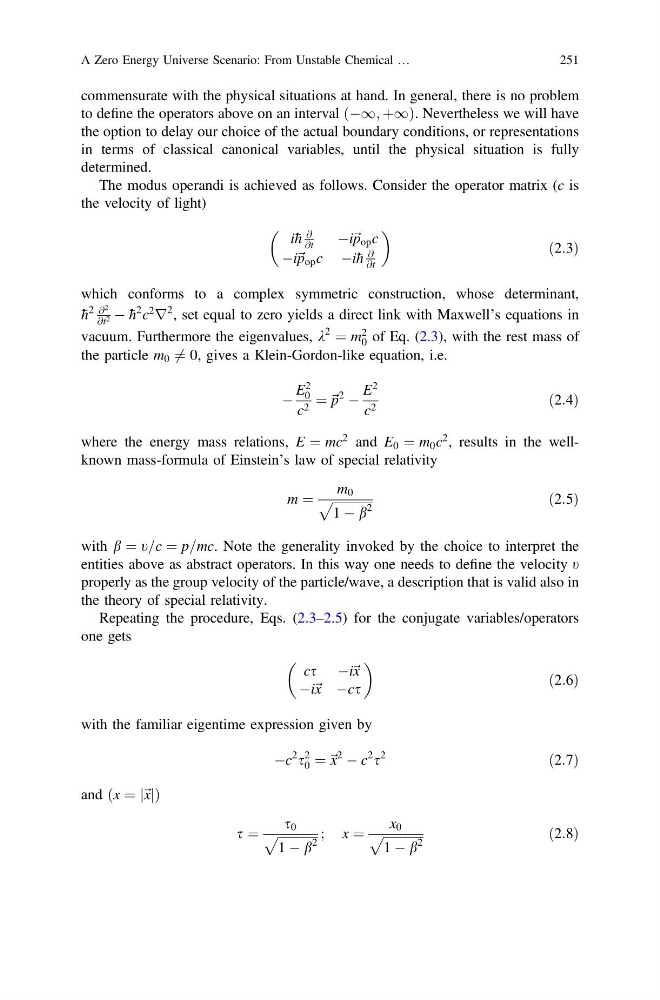
commensurate with the physical situations at hand. In general, there is no problem
to define the operators above on an interval À1; þ1
ð
Þ . Nevertheless we will have
the option to delay our choice of the actual boundary conditions, or representations
in terms of classical canonical variables, until the physical situation is fully
determined.
The modus operandi is achieved as follows. Consider the operator matrix (c is
the velocity of light)
i h
@
@t
Ài~ p op c
Ài~ p op c Ài h
@
@t
ð2:3Þ
which conforms to a complex symmetric construction, whose determinant,
h
2 @
2
@t 2 À h
2 c
2
r
2 , set equal to zero yields a direct link with Maxwell’s equations in
vacuum. Furthermore the eigenvalues, k
2
¼ m
2
0 of Eq. (2.3), with the rest mass of
the particle m 0 6 ¼ 0, gives a Klein-Gordon-like equation, i.e.
À
E
2
0
c 2 ¼ ~ p
2
À
E
2
c 2
ð2:4Þ
where the energy mass relations, E ¼ mc
2 and E 0 ¼ m 0 c
2 , results in the wellknown mass-formula of Einstein’s law of special relativity
m ¼
m 0
ffiffiffiffiffiffiffiffiffiffiffiffiffi
1 À b
2
p
ð2:5Þ
with b ¼ t=c ¼ p=mc. Note the generality invoked by the choice to interpret the
entities above as abstract operators. In this way one needs to define the velocity t
properly as the group velocity of the particle/wave, a description that is valid also in
the theory of special relativity.
Repeating the procedure, Eqs. (2.3–2.5) for the conjugate variables/operators
one gets
cs Ài~ x
Ài~ x Àcs
ð2:6Þ
with the familiar eigentime expression given by
Àc
2
s
2
0 ¼ ~ x
2
À c
2
s
2
ð2:7Þ
and x ¼ j~ xj
ð
Þ
s ¼
s 0
ffiffiffiffiffiffiffiffiffiffiffiffiffi
1 À b
2
p
; x ¼
x 0
ffiffiffiffiffiffiffiffiffiffiffiffiffi
1 À b
2
p
ð2:8Þ
A Zero Energy Universe Scenario: From Unstable Chemical …
251