

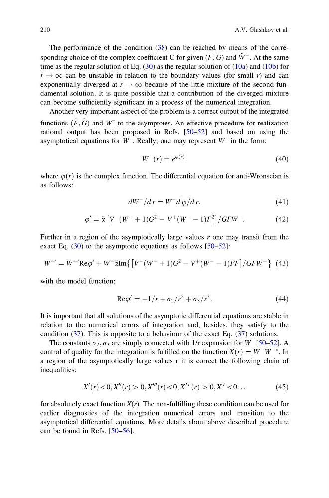
The performance of the condition (38) can be reached by means of the corresponding choice of the complex coefficient C for given (F, G) and ~
W
À . At the same
time as the regular solution of Eq. (30) as the regular solution of (10a) and (10b) for
r ! 1 can be unstable in relation to the boundary values (for small r) and can
exponentially diverged at r ! 1 because of the little mixture of the second fundamental solution. It is quite possible that a contribution of the diverged mixture
can become sufficiently significant in a process of the numerical integration.
Another very important aspect of the problem is a correct output of the integrated
functions ðF
_ ; G
_ Þ and W
− to the asymptotes. An effective procedure for realization
rational output has been proposed in Refs. [50–52] and based on using the
asymptotical equations for W
− . Really, one may represent W
− in the form:
W
À
ðrÞ ¼ e
uðrÞ
:
ð40Þ
where uðrÞ is the complex function. The differential equation for anti-Wronscian is
as follows:
dW
À
=d r ¼ W
À d u=d r:
ð41Þ
u
0
¼ ~ a V
À W
À
þ 1
ð
Þ G
2
À V
þ W
À
À 1
ð
Þ F
2
Â
à =GFW
À
:
ð42Þ
Further in a region of the asymptotically large values r one may transit from the
exact Eq. (30) to the asymptotic equations as follows [50–52]:
W
À0
¼ W
À0 Reu
0
þ W
À
~ aIm V
À W
À
þ 1
ð
Þ G
2
À V
þ W
À
À 1
ð
Þ FF
Â
à =GFW
À
È
É ð43Þ
with the model function:
Reu
0
¼ À1=r þ r 2 =r
2
þ r 3 =r
3
:
ð44Þ
It is important that all solutions of the asymptotic differential equations are stable in
relation to the numerical errors of integration and, besides, they satisfy to the
condition (37). This is opposite to a behaviour of the exact Eq. (37) solutions.
The constants r 2 ; r 3 are simply connected with 1/r expansion for W
− [50–52]. A
control of quality for the integration is fulfilled on the function XðrÞ ¼ W
À W
ÀÃ . In
a region of the asymptotically large values r it is correct the following chain of
inequalities:
X
0
ðrÞ\0; X
00
ðrÞ [ 0; X
000
ðrÞ\0; X
IV
ðrÞ [ 0; X
V
\0. . .
ð45Þ
for absolutely exact function X(r). The non-fulfilling these condition can be used for
earlier diagnostics of the integration numerical errors and transition to the
asymptotical differential equations. More details about above described procedure
can be found in Refs. [50–56].
210
A.V. Glushkov et al.
W
À . At the same
time as the regular solution of Eq. (30) as the regular solution of (10a) and (10b) for
r ! 1 can be unstable in relation to the boundary values (for small r) and can
exponentially diverged at r ! 1 because of the little mixture of the second fundamental solution. It is quite possible that a contribution of the diverged mixture
can become sufficiently significant in a process of the numerical integration.
Another very important aspect of the problem is a correct output of the integrated
functions ðF
_ ; G
_ Þ and W
− to the asymptotes. An effective procedure for realization
rational output has been proposed in Refs. [50–52] and based on using the
asymptotical equations for W
− . Really, one may represent W
− in the form:
W
À
ðrÞ ¼ e
uðrÞ
:
ð40Þ
where uðrÞ is the complex function. The differential equation for anti-Wronscian is
as follows:
dW
À
=d r ¼ W
À d u=d r:
ð41Þ
u
0
¼ ~ a V
À W
À
þ 1
ð
Þ G
2
À V
þ W
À
À 1
ð
Þ F
2
Â
à =GFW
À
:
ð42Þ
Further in a region of the asymptotically large values r one may transit from the
exact Eq. (30) to the asymptotic equations as follows [50–52]:
W
À0
¼ W
À0 Reu
0
þ W
À
~ aIm V
À W
À
þ 1
ð
Þ G
2
À V
þ W
À
À 1
ð
Þ FF
Â
à =GFW
À
È
É ð43Þ
with the model function:
Reu
0
¼ À1=r þ r 2 =r
2
þ r 3 =r
3
:
ð44Þ
It is important that all solutions of the asymptotic differential equations are stable in
relation to the numerical errors of integration and, besides, they satisfy to the
condition (37). This is opposite to a behaviour of the exact Eq. (37) solutions.
The constants r 2 ; r 3 are simply connected with 1/r expansion for W
− [50–52]. A
control of quality for the integration is fulfilled on the function XðrÞ ¼ W
À W
ÀÃ . In
a region of the asymptotically large values r it is correct the following chain of
inequalities:
X
0
ðrÞ\0; X
00
ðrÞ [ 0; X
000
ðrÞ\0; X
IV
ðrÞ [ 0; X
V
\0. . .
ð45Þ
for absolutely exact function X(r). The non-fulfilling these condition can be used for
earlier diagnostics of the integration numerical errors and transition to the
asymptotical differential equations. More details about above described procedure
can be found in Refs. [50–56].
210
A.V. Glushkov et al.