350 Appendix 2: Product Upgrades Based on Minimum Expected Quality Loss
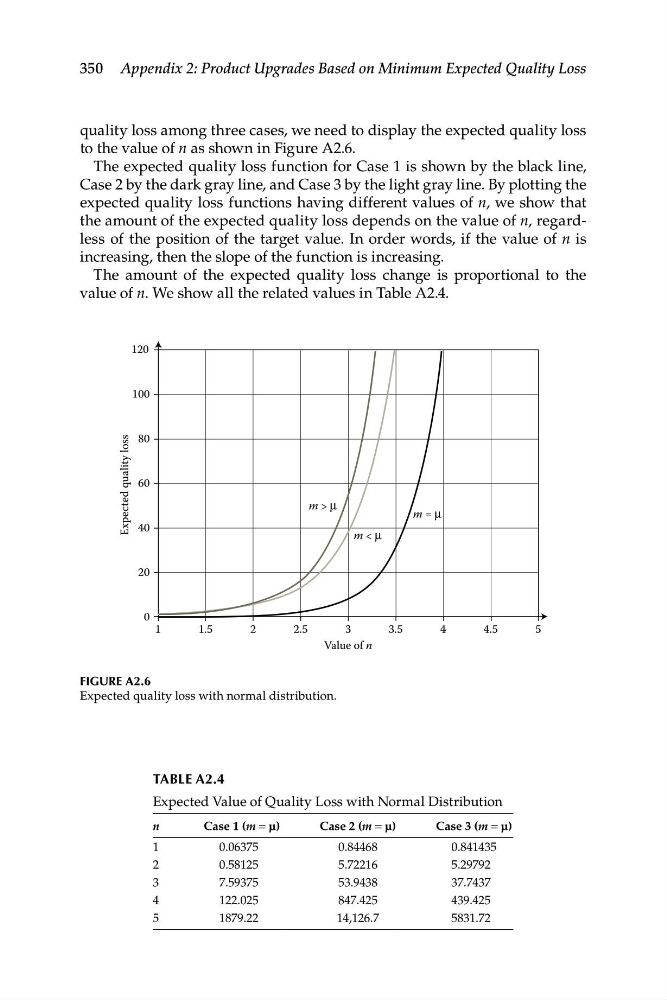
quality loss among three cases, we need to display the expected quality loss
to the value of n as shown in Figure A2.6.
The expected quality loss function for Case 1 is shown by the black line,
Case 2 by the dark gray line, and Case 3 by the light gray line. By plotting the
expected quality loss functions having different values of n, we show that
the amount of the expected quality loss depends on the value of n, regard
less of the position of the target value. In order words, if the value of n is
increasing, then the slope of the function is increasing.
The amount of the expected quality loss change is proportional to the
value of n. We show all the related values in Table A2.4.
­
1
0
20
40
60
80
100
1.5
2
2.5
3
3.5
m > μ
m < μ
m = μ
4
4.5
120
5
Expected quality loss
Value of n
FIgure A2.6
Expected quality loss with normal distribution.
TABLe A2.4
Expected Value of Quality Loss with Normal Distribution
n
Case 1 (m = μ)
Case 2 (m = μ)
Case 3 (m = μ)
1
0.06375
0.84468
0.841435
2
0.58125
5.72216
5.29792
3
7.59375
53.9438
37.7437
4
122.025
847.425
439.425
5
1879.22
14,126.7
5831.72