

349
Appendix 2: Product Upgrades Based on Minimum Expected Quality Loss
In order to show the trend of the expected quality loss according to the
position of the target value, we consider three cases of the mean of quality
output, by using a numerical example.
Case 1: the target value of the quality characteristic is equal to the mean
of quality.
Case 2: the target value of the quality characteristic is greater than the
mean of quality.
Case 3: the target value is less than the mean of quality.
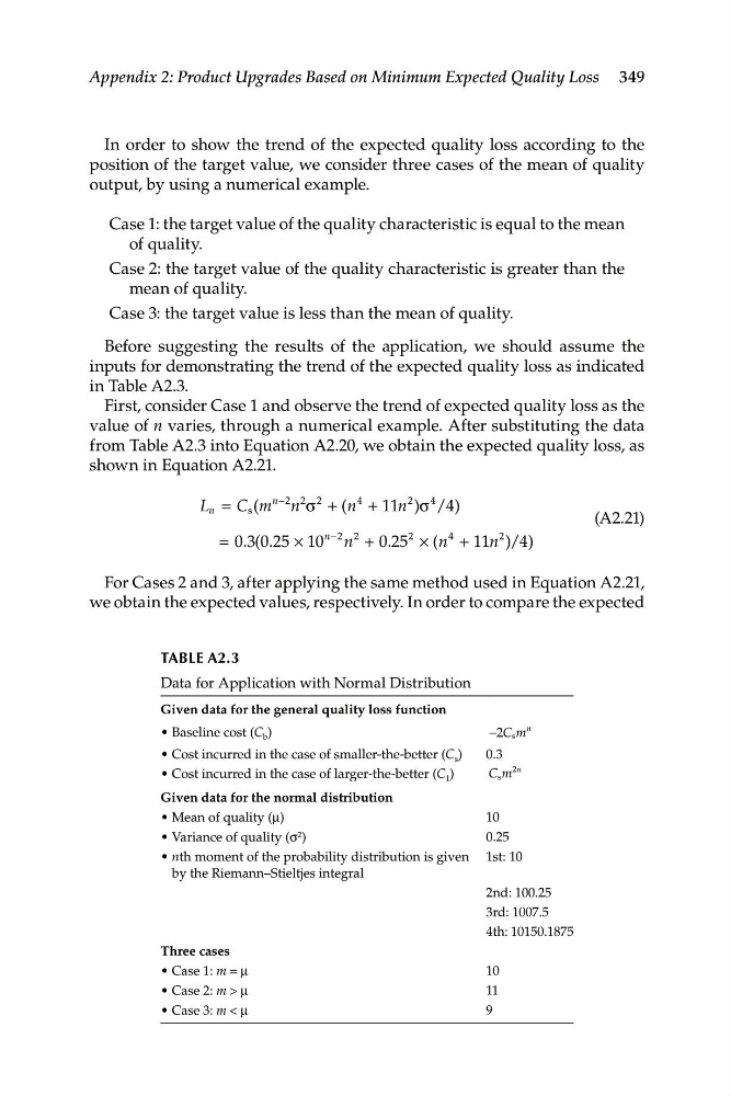
Before suggesting the results of the application, we should assume the
inputs for demonstrating the trend of the expected quality loss as indicated
in Table A2.3.
First, consider Case 1 and observe the trend of expected quality loss as the
value of n varies, through a numerical example. After substituting the data
from Table A2.3 into Equation A2.20, we obtain the expected quality loss, as
shown in Equation A2.21.
L = C (m
n−2 n
2 2
+ n
4
+ n
2
4
n
s
σ
(
11 )σ /4)
(A2.21)
= 0.3(0.25 × 10
n−2 n
2
+ 0.25
2
× (n
4
+ 11 1n
2 )/4)
For Cases 2 and 3, after applying the same method used in Equation A2.21,
we obtain the expected values, respectively. In order to compare the expected
TABLe A2.3
Data for Application with Normal Distribution
Given data for the general quality loss function
• Baseline cost (C b )
• Cost incurred in the case of smaller-the-better (C s )
• Cost incurred in the case of larger-the-better (C 1 )
Given data for the normal distribution
• Mean of quality (μ)
• Variance of quality (σ 2 )
• nth moment of the probability distribution is given
by the Riemann–Stieltjes integral
Three cases
• Case 1: m = μ
• Case 2: m > μ
• Case 3: m < μ
n
−2C m
s
0.3
2n
C m
s
10
0.25
1st: 10
2nd: 100.25
3rd: 1007.5
4th: 10150.1875
10
11
9
Appendix 2: Product Upgrades Based on Minimum Expected Quality Loss
In order to show the trend of the expected quality loss according to the
position of the target value, we consider three cases of the mean of quality
output, by using a numerical example.
Case 1: the target value of the quality characteristic is equal to the mean
of quality.
Case 2: the target value of the quality characteristic is greater than the
mean of quality.
Case 3: the target value is less than the mean of quality.
Before suggesting the results of the application, we should assume the
inputs for demonstrating the trend of the expected quality loss as indicated
in Table A2.3.
First, consider Case 1 and observe the trend of expected quality loss as the
value of n varies, through a numerical example. After substituting the data
from Table A2.3 into Equation A2.20, we obtain the expected quality loss, as
shown in Equation A2.21.
L = C (m
n−2 n
2 2
+ n
4
+ n
2
4
n
s
σ
(
11 )σ /4)
(A2.21)
= 0.3(0.25 × 10
n−2 n
2
+ 0.25
2
× (n
4
+ 11 1n
2 )/4)
For Cases 2 and 3, after applying the same method used in Equation A2.21,
we obtain the expected values, respectively. In order to compare the expected
TABLe A2.3
Data for Application with Normal Distribution
Given data for the general quality loss function
• Baseline cost (C b )
• Cost incurred in the case of smaller-the-better (C s )
• Cost incurred in the case of larger-the-better (C 1 )
Given data for the normal distribution
• Mean of quality (μ)
• Variance of quality (σ 2 )
• nth moment of the probability distribution is given
by the Riemann–Stieltjes integral
Three cases
• Case 1: m = μ
• Case 2: m > μ
• Case 3: m < μ
n
−2C m
s
0.3
2n
C m
s
10
0.25
1st: 10
2nd: 100.25
3rd: 1007.5
4th: 10150.1875
10
11
9