

is given by the variogram, cf. Fig. 22.11d), the
model values will tend towards the average. There
will only be one single outcome “realisation” in
kriging mode. An important weakness with kriging
is that the result becomes too smooth, and therefore
unsuitable for realistic flow modelling.
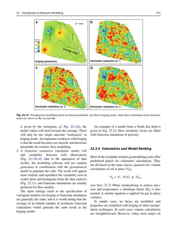
2. A Gaussian simulation (stochastic mode) will
add variability between well observations
(Fig. 22.13b–d). Due to the sparseness of data
(wells), the modelling software will use random
generators in combination with the geostatistical
model to populate the cells. The result will appear
more realistic and reproduce the variability seen in
scatter plots and histograms from the data analysis
(Fig. 22.11), and Gaussian simulations are usually
preferred for flow models.
The input settings (such as the specification of
variogram models) for kriging or Gaussian simulation
are generally the same, and it is worth noting that the
average of an infinite number of stochastic Gaussian
realisations would generate the same result as the
kriging model.
An example of a model from a North Sea field is
given in Fig. 22.14. Here stochastic facies are filled
with Gaussian simulation of porosity.
22.3.4 Volumetrics and Model Ranking
Most of the available modern geomodelling tools offer
predefined panels for volumetric calculations. They
are all based on the same classic equations for volume
calculations of oil in place (V p )
V p ¼ V r Á N=G Á φ Á O sat
(see Sect. 21.2) When standardising to surface pressure and temperature, a shrinkage factor (B o ) is also
needed. A similar equation is applied for gas in place
volumes.
In simple cases, no facies are modelled, and
properties are modelled with kriging or other interpolation techniques. In such cases volume calculations
are straightforward. However, today most major oil
Fig. 22.13 Petrophysical modelling based on Gaussian methods. (a) Shows kriging mode, while three realisations from stochastic
mode are shown in (b), (c) and (d)
22 Introduction to Reservoir Modelling
573
model values will tend towards the average. There
will only be one single outcome “realisation” in
kriging mode. An important weakness with kriging
is that the result becomes too smooth, and therefore
unsuitable for realistic flow modelling.
2. A Gaussian simulation (stochastic mode) will
add variability between well observations
(Fig. 22.13b–d). Due to the sparseness of data
(wells), the modelling software will use random
generators in combination with the geostatistical
model to populate the cells. The result will appear
more realistic and reproduce the variability seen in
scatter plots and histograms from the data analysis
(Fig. 22.11), and Gaussian simulations are usually
preferred for flow models.
The input settings (such as the specification of
variogram models) for kriging or Gaussian simulation
are generally the same, and it is worth noting that the
average of an infinite number of stochastic Gaussian
realisations would generate the same result as the
kriging model.
An example of a model from a North Sea field is
given in Fig. 22.14. Here stochastic facies are filled
with Gaussian simulation of porosity.
22.3.4 Volumetrics and Model Ranking
Most of the available modern geomodelling tools offer
predefined panels for volumetric calculations. They
are all based on the same classic equations for volume
calculations of oil in place (V p )
V p ¼ V r Á N=G Á φ Á O sat
(see Sect. 21.2) When standardising to surface pressure and temperature, a shrinkage factor (B o ) is also
needed. A similar equation is applied for gas in place
volumes.
In simple cases, no facies are modelled, and
properties are modelled with kriging or other interpolation techniques. In such cases volume calculations
are straightforward. However, today most major oil
Fig. 22.13 Petrophysical modelling based on Gaussian methods. (a) Shows kriging mode, while three realisations from stochastic
mode are shown in (b), (c) and (d)
22 Introduction to Reservoir Modelling
573