

based methods place the various facies bodies into a
background facies, according to statistical rules and
geometrical relationships. Object modelling is intuitive in the way that input is provided by the modeller
on the shape and size of the objects to be modelled, but
may be complex to parameterise and to condition (fit)
with all observations, such as blocked wells and seismic data. Sometimes the methods are slow to run
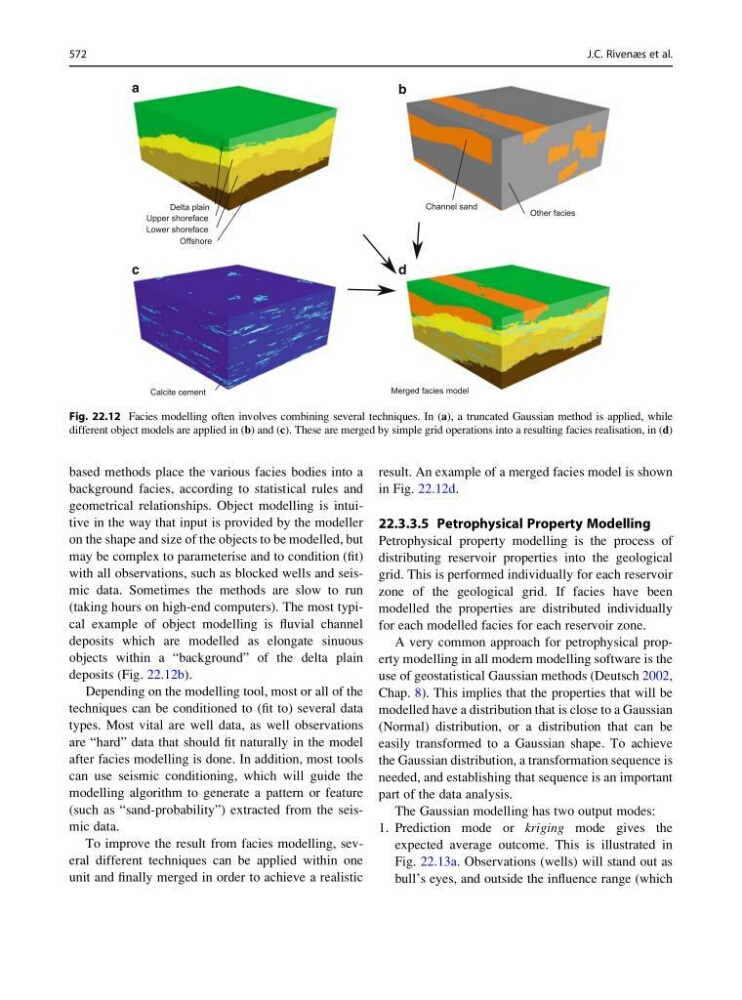
(taking hours on high-end computers). The most typical example of object modelling is fluvial channel
deposits which are modelled as elongate sinuous
objects within a “background” of the delta plain
deposits (Fig. 22.12b).
Depending on the modelling tool, most or all of the
techniques can be conditioned to (fit to) several data
types. Most vital are well data, as well observations
are “hard” data that should fit naturally in the model
after facies modelling is done. In addition, most tools
can use seismic conditioning, which will guide the
modelling algorithm to generate a pattern or feature
(such as “sand-probability”) extracted from the seismic data.
To improve the result from facies modelling, several different techniques can be applied within one
unit and finally merged in order to achieve a realistic
result. An example of a merged facies model is shown
in Fig. 22.12d.
22.3.3.5 Petrophysical Property Modelling
Petrophysical property modelling is the process of
distributing reservoir properties into the geological
grid. This is performed individually for each reservoir
zone of the geological grid. If facies have been
modelled the properties are distributed individually
for each modelled facies for each reservoir zone.
A very common approach for petrophysical property modelling in all modern modelling software is the
use of geostatistical Gaussian methods (Deutsch 2002,
Chap. 8). This implies that the properties that will be
modelled have a distribution that is close to a Gaussian
(Normal) distribution, or a distribution that can be
easily transformed to a Gaussian shape. To achieve
the Gaussian distribution, a transformation sequence is
needed, and establishing that sequence is an important
part of the data analysis.
The Gaussian modelling has two output modes:
1. Prediction mode or kriging mode gives the
expected average outcome. This is illustrated in
Fig. 22.13a. Observations (wells) will stand out as
bull’s eyes, and outside the influence range (which
a
b
c
d
Fig. 22.12 Facies modelling often involves combining several techniques. In (a), a truncated Gaussian method is applied, while
different object models are applied in (b) and (c). These are merged by simple grid operations into a resulting facies realisation, in (d)
572
J.C. Rivenæs et al.
background facies, according to statistical rules and
geometrical relationships. Object modelling is intuitive in the way that input is provided by the modeller
on the shape and size of the objects to be modelled, but
may be complex to parameterise and to condition (fit)
with all observations, such as blocked wells and seismic data. Sometimes the methods are slow to run
(taking hours on high-end computers). The most typical example of object modelling is fluvial channel
deposits which are modelled as elongate sinuous
objects within a “background” of the delta plain
deposits (Fig. 22.12b).
Depending on the modelling tool, most or all of the
techniques can be conditioned to (fit to) several data
types. Most vital are well data, as well observations
are “hard” data that should fit naturally in the model
after facies modelling is done. In addition, most tools
can use seismic conditioning, which will guide the
modelling algorithm to generate a pattern or feature
(such as “sand-probability”) extracted from the seismic data.
To improve the result from facies modelling, several different techniques can be applied within one
unit and finally merged in order to achieve a realistic
result. An example of a merged facies model is shown
in Fig. 22.12d.
22.3.3.5 Petrophysical Property Modelling
Petrophysical property modelling is the process of
distributing reservoir properties into the geological
grid. This is performed individually for each reservoir
zone of the geological grid. If facies have been
modelled the properties are distributed individually
for each modelled facies for each reservoir zone.
A very common approach for petrophysical property modelling in all modern modelling software is the
use of geostatistical Gaussian methods (Deutsch 2002,
Chap. 8). This implies that the properties that will be
modelled have a distribution that is close to a Gaussian
(Normal) distribution, or a distribution that can be
easily transformed to a Gaussian shape. To achieve
the Gaussian distribution, a transformation sequence is
needed, and establishing that sequence is an important
part of the data analysis.
The Gaussian modelling has two output modes:
1. Prediction mode or kriging mode gives the
expected average outcome. This is illustrated in
Fig. 22.13a. Observations (wells) will stand out as
bull’s eyes, and outside the influence range (which
a
b
c
d
Fig. 22.12 Facies modelling often involves combining several techniques. In (a), a truncated Gaussian method is applied, while
different object models are applied in (b) and (c). These are merged by simple grid operations into a resulting facies realisation, in (d)
572
J.C. Rivenæs et al.