

geomodelling perspective but especially from a dynamic
simulation point of view. The maximum number of grid
cells in a model is limited by prevailing computer
power, but as an estimate static models can handle
up to 100 million cells which is typically two orders
of magnitude more than dynamic models can deal
with. There are a few important requirements
concerning the geological modelling grid:
• The grid should be as uniform as possible, hence
the grid cell size should not vary too much in the
model, for each zone. The underlying methods for
property modelling commonly assume a uniform
grid, and the result may be distorted if the grid is
non-uniform.
• The grid orientation both vertically and laterally
should follow main directions of the heterogeneities.
It is important to have a good multidisciplinary
co-operation when designing the geological modelling
grid, taking into account not only the input parameters
but also the modelling objectives and practical use of
the grid. A simple grid (i.e. coarser grid resolution and
fewer grid cells) designed for a crude in-place volume
estimates will have quite different requirements relative to a grid constructed for a static model that shall
serve as basis for a dynamic simulation model for the
calculation of production profiles and reservoir
management.
22.3.3 Property Modelling
When the grid construction is finished, the next step is
to fill in the cells with properties. The most important
properties are the petrophysical ones (porosity,
permeabilities, saturations), but the grid may contain
a large number of properties. We can classify the
properties into two main categories:
Discrete or Categorical Properties These properties
hold a single integer value per cell. This cell value is
commonly just an alias or indicator for a given feature,
such as a facies name. For example, cells with integer
value 1 may be associated with facies “channel-sand”,
while cells with value 2 may be associated with facies
“deltaplain-mudstone”, etc. The use of numbers and
associated facies names will vary from case to case.
Other examples of discrete variables are region and
fault block identifiers.
Continuous Properties These values represent a scalar representation of a petrophysical property directly,
such as porosity (which is usually given in a fractional
a
b
c
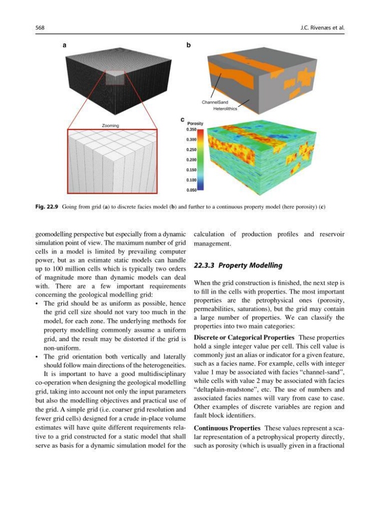
Fig. 22.9 Going from grid (a) to discrete facies model (b) and further to a continuous property model (here porosity) (c)
568
J.C. Rivenæs et al.
simulation point of view. The maximum number of grid
cells in a model is limited by prevailing computer
power, but as an estimate static models can handle
up to 100 million cells which is typically two orders
of magnitude more than dynamic models can deal
with. There are a few important requirements
concerning the geological modelling grid:
• The grid should be as uniform as possible, hence
the grid cell size should not vary too much in the
model, for each zone. The underlying methods for
property modelling commonly assume a uniform
grid, and the result may be distorted if the grid is
non-uniform.
• The grid orientation both vertically and laterally
should follow main directions of the heterogeneities.
It is important to have a good multidisciplinary
co-operation when designing the geological modelling
grid, taking into account not only the input parameters
but also the modelling objectives and practical use of
the grid. A simple grid (i.e. coarser grid resolution and
fewer grid cells) designed for a crude in-place volume
estimates will have quite different requirements relative to a grid constructed for a static model that shall
serve as basis for a dynamic simulation model for the
calculation of production profiles and reservoir
management.
22.3.3 Property Modelling
When the grid construction is finished, the next step is
to fill in the cells with properties. The most important
properties are the petrophysical ones (porosity,
permeabilities, saturations), but the grid may contain
a large number of properties. We can classify the
properties into two main categories:
Discrete or Categorical Properties These properties
hold a single integer value per cell. This cell value is
commonly just an alias or indicator for a given feature,
such as a facies name. For example, cells with integer
value 1 may be associated with facies “channel-sand”,
while cells with value 2 may be associated with facies
“deltaplain-mudstone”, etc. The use of numbers and
associated facies names will vary from case to case.
Other examples of discrete variables are region and
fault block identifiers.
Continuous Properties These values represent a scalar representation of a petrophysical property directly,
such as porosity (which is usually given in a fractional
a
b
c
Fig. 22.9 Going from grid (a) to discrete facies model (b) and further to a continuous property model (here porosity) (c)
568
J.C. Rivenæs et al.