

22.3.1 Seismic and Geological Framework
The seismic framework typically defines the top and
base reservoir and in some cases internal reflectors
(Fig. 22.6, steps a–d). Faults are interpreted from
discontinuities in the seismic reflectors. As the seismic
interpretation usually is done in the Two-Way Time
(TWT) domain, a depth conversion will be needed. As
the seismic resolution usually is limited to a few
horizons in the reservoir, additional zones are commonly added based on well correlation (supported by
the conceptual model). This provides the basis for
creating isochore (thickness) maps, which are merged
into the seismic framework (including faults) by the
modelling software. The resulting mix of interpreted
seismic surfaces, faults and calculated intermediate
horizons from well correlation and isochores makes
the geological framework, which can be considered as
the most precise model of the structural elements
(Fig. 22.6, steps e–h). Note that different modelling
software has different approaches to the details of this
work flow, and some software incorporates parts of
zonal modelling directly in the 3D gridding process.
22.3.2 3D Gridding for Static Modelling
The geological framework (comprising interpreted
and calculated horizons) is usually surface oriented,
i.e. it is made by a number of maps which make up a
skeleton in three dimensions. However, properties
may have values in any position between the surfaces.
In order to populate the digital model with properties,
we introduce an additional data type: the 3D grid. The
3D grid consists of numerous cells to build the reservoir volume, analogue to a “flexible” Lego brick
model, and we often refer to this a geocellular
model. What is important to understand in the property
modelling is that each grid cell in the model is
assigned one value for each reservoir property to be
modelled. The typical size for a grid cell is from 20 m
to a few hundred metres lateral resolution (X and Y
direction of grid) and 0.5 m to up to 10’s of metres
vertical resolution (Z direction of grid); hence
petrophysical values are averaged over a much larger
volume than primary input such as core plugs and
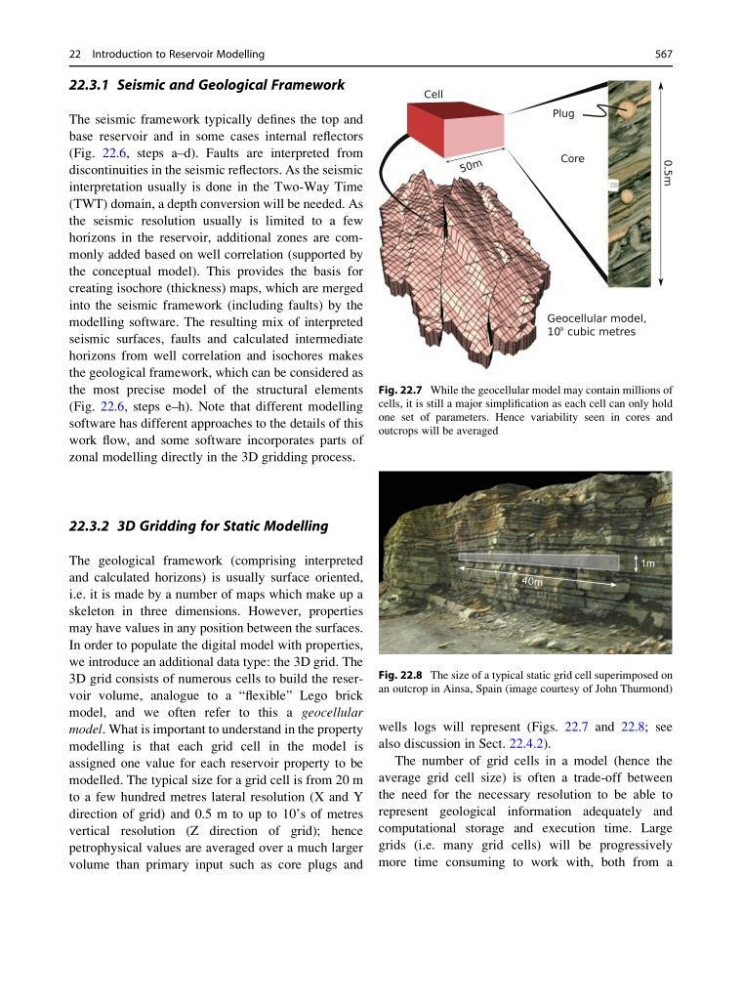
wells logs will represent (Figs. 22.7 and 22.8; see
also discussion in Sect. 22.4.2).
The number of grid cells in a model (hence the
average grid cell size) is often a trade-off between
the need for the necessary resolution to be able to
represent geological information adequately and
computational storage and execution time. Large
grids (i.e. many grid cells) will be progressively
more time consuming to work with, both from a
Fig. 22.7 While the geocellular model may contain millions of
cells, it is still a major simplification as each cell can only hold
one set of parameters. Hence variability seen in cores and
outcrops will be averaged
Fig. 22.8 The size of a typical static grid cell superimposed on
an outcrop in Ainsa, Spain (image courtesy of John Thurmond)
22 Introduction to Reservoir Modelling
567
The seismic framework typically defines the top and
base reservoir and in some cases internal reflectors
(Fig. 22.6, steps a–d). Faults are interpreted from
discontinuities in the seismic reflectors. As the seismic
interpretation usually is done in the Two-Way Time
(TWT) domain, a depth conversion will be needed. As
the seismic resolution usually is limited to a few
horizons in the reservoir, additional zones are commonly added based on well correlation (supported by
the conceptual model). This provides the basis for
creating isochore (thickness) maps, which are merged
into the seismic framework (including faults) by the
modelling software. The resulting mix of interpreted
seismic surfaces, faults and calculated intermediate
horizons from well correlation and isochores makes
the geological framework, which can be considered as
the most precise model of the structural elements
(Fig. 22.6, steps e–h). Note that different modelling
software has different approaches to the details of this
work flow, and some software incorporates parts of
zonal modelling directly in the 3D gridding process.
22.3.2 3D Gridding for Static Modelling
The geological framework (comprising interpreted
and calculated horizons) is usually surface oriented,
i.e. it is made by a number of maps which make up a
skeleton in three dimensions. However, properties
may have values in any position between the surfaces.
In order to populate the digital model with properties,
we introduce an additional data type: the 3D grid. The
3D grid consists of numerous cells to build the reservoir volume, analogue to a “flexible” Lego brick
model, and we often refer to this a geocellular
model. What is important to understand in the property
modelling is that each grid cell in the model is
assigned one value for each reservoir property to be
modelled. The typical size for a grid cell is from 20 m
to a few hundred metres lateral resolution (X and Y
direction of grid) and 0.5 m to up to 10’s of metres
vertical resolution (Z direction of grid); hence
petrophysical values are averaged over a much larger
volume than primary input such as core plugs and
wells logs will represent (Figs. 22.7 and 22.8; see
also discussion in Sect. 22.4.2).
The number of grid cells in a model (hence the
average grid cell size) is often a trade-off between
the need for the necessary resolution to be able to
represent geological information adequately and
computational storage and execution time. Large
grids (i.e. many grid cells) will be progressively
more time consuming to work with, both from a
Fig. 22.7 While the geocellular model may contain millions of
cells, it is still a major simplification as each cell can only hold
one set of parameters. Hence variability seen in cores and
outcrops will be averaged
Fig. 22.8 The size of a typical static grid cell superimposed on
an outcrop in Ainsa, Spain (image courtesy of John Thurmond)
22 Introduction to Reservoir Modelling
567