

20.2.6.1 Electrical Anisotropy
Sediments and layered strata can be strongly electrically anisotropic. This is a combination of intrinsic
anisotropy (e.g. anisotropy within the shale) and
large-scale anisotropy (e.g. anisotropy due to thin
bed layering). If anisotropy is not taken into account
it can easily lead to false inversion- and interpretation
results. Most forward modelling and inversion
algorithms assume a TIV media (Transverse Isotropic
with a Vertical axis of symmetry). This means that
electrical properties of subsurface rocks are described
by a horizontal and a vertical resistivity component.
The anisotropy is defined as the vertical divided by the
horizontal resistivity component. Typically, vertical
resistivity will often be higher than horizontal resistivity due to the horizontal layering of beds and strata.
Today most resistivity well log tools only measure the
horizontal resistivity. In such cases it is only possible
to directly calibrate the horizontal resistivity model to
the well logs.
When tri-axial resistivity logging tools measuring
both directions become more common, calibration
also of the vertical resistivity model derived from
CSEM data will be possible. Better understanding of
the electrical anisotropy will improve our ability to
interpret CSEM data.
20.2.6.2 Apparent Anisotropy
As explained above, 3D CSEM acquisition provides
both inline- and broadside data. The inline data is
sensitive to the vertical resistivity (Rv) in the Earth,
while the broadside data is sensitive to the horizontal
resistivity (Rh) in the subsurface. Azimuthal data
measures both inline and broadside data, and is therefore sensitive to both horizontal and vertical
resistivity.
In addition it is only the in-line data that is sensitive
to thin horizontal resistive layers. The broadside data
is not able to detect thin horizontal resistive layers, but
measures background resistivity trends. This is
because horizontal currents will flow around a thin
resistor while vertical currents will not. The situation
is opposite for thin vertical resistors. Here vertical
currents can flow around the resistor while horizontal
current will not. In this case the vertical resistor will be
imaged better in the horizontal resistivity model than
in the vertical resistivity model.
The difference in sensitivity can be illustrated by
using a synthetic example (Fig. 20.12). The upper
panels show the Earth model’s vertical (left column)
and horizontal resistivity (right column). The thin
resistor (red target) is a hydrocarbon reservoir with
equally high vertical and horizontal resistivity.
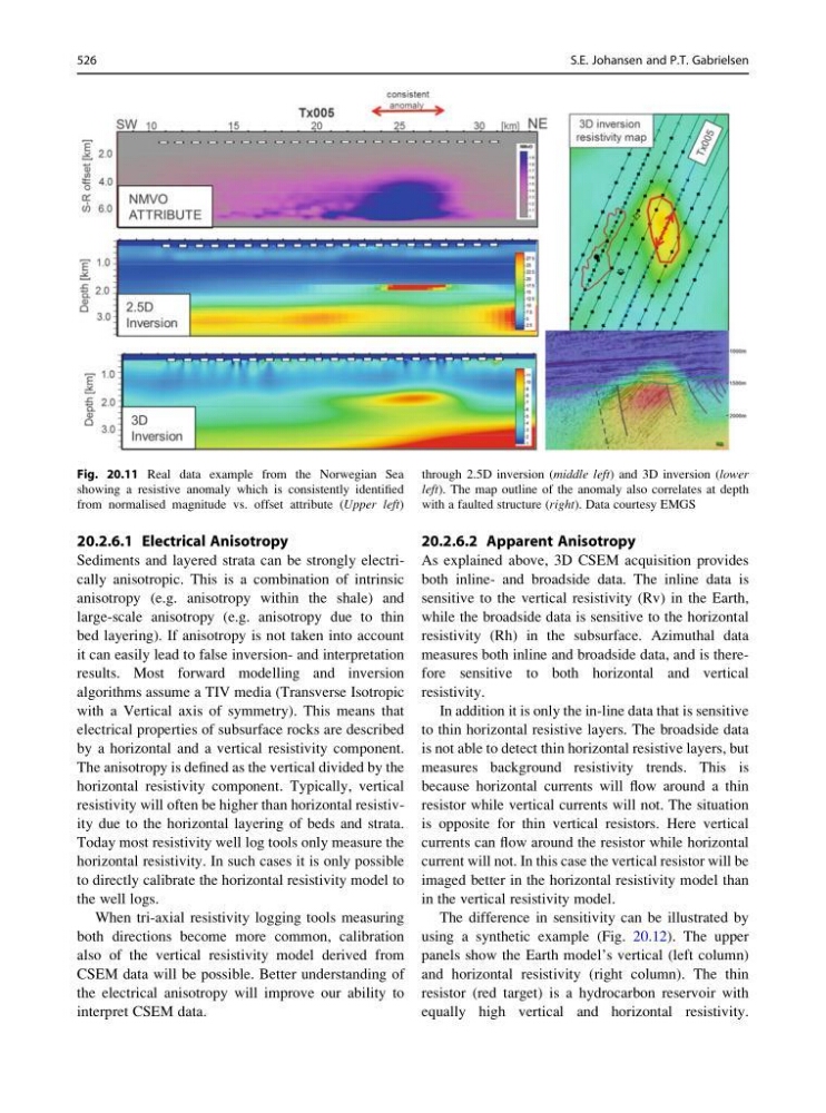
Fig. 20.11 Real data example from the Norwegian Sea
showing a resistive anomaly which is consistently identified
from normalised magnitude vs. offset attribute (Upper left)
through 2.5D inversion (middle left) and 3D inversion (lower
left). The map outline of the anomaly also correlates at depth
with a faulted structure (right). Data courtesy EMGS
526
S.E. Johansen and P.T. Gabrielsen
Sediments and layered strata can be strongly electrically anisotropic. This is a combination of intrinsic
anisotropy (e.g. anisotropy within the shale) and
large-scale anisotropy (e.g. anisotropy due to thin
bed layering). If anisotropy is not taken into account
it can easily lead to false inversion- and interpretation
results. Most forward modelling and inversion
algorithms assume a TIV media (Transverse Isotropic
with a Vertical axis of symmetry). This means that
electrical properties of subsurface rocks are described
by a horizontal and a vertical resistivity component.
The anisotropy is defined as the vertical divided by the
horizontal resistivity component. Typically, vertical
resistivity will often be higher than horizontal resistivity due to the horizontal layering of beds and strata.
Today most resistivity well log tools only measure the
horizontal resistivity. In such cases it is only possible
to directly calibrate the horizontal resistivity model to
the well logs.
When tri-axial resistivity logging tools measuring
both directions become more common, calibration
also of the vertical resistivity model derived from
CSEM data will be possible. Better understanding of
the electrical anisotropy will improve our ability to
interpret CSEM data.
20.2.6.2 Apparent Anisotropy
As explained above, 3D CSEM acquisition provides
both inline- and broadside data. The inline data is
sensitive to the vertical resistivity (Rv) in the Earth,
while the broadside data is sensitive to the horizontal
resistivity (Rh) in the subsurface. Azimuthal data
measures both inline and broadside data, and is therefore sensitive to both horizontal and vertical
resistivity.
In addition it is only the in-line data that is sensitive
to thin horizontal resistive layers. The broadside data
is not able to detect thin horizontal resistive layers, but
measures background resistivity trends. This is
because horizontal currents will flow around a thin
resistor while vertical currents will not. The situation
is opposite for thin vertical resistors. Here vertical
currents can flow around the resistor while horizontal
current will not. In this case the vertical resistor will be
imaged better in the horizontal resistivity model than
in the vertical resistivity model.
The difference in sensitivity can be illustrated by
using a synthetic example (Fig. 20.12). The upper
panels show the Earth model’s vertical (left column)
and horizontal resistivity (right column). The thin
resistor (red target) is a hydrocarbon reservoir with
equally high vertical and horizontal resistivity.
Fig. 20.11 Real data example from the Norwegian Sea
showing a resistive anomaly which is consistently identified
from normalised magnitude vs. offset attribute (Upper left)
through 2.5D inversion (middle left) and 3D inversion (lower
left). The map outline of the anomaly also correlates at depth
with a faulted structure (right). Data courtesy EMGS
526
S.E. Johansen and P.T. Gabrielsen